March 2026
Maxwell’s equations in vacuum are governed by two independent electromagnetic invariants: the propagation speed \(c\) and the impedance \(Z_0= \sqrt{\mu_0/\varepsilon_0}\). Atomic physics has used \(c\) extensively. We show that \(Z_0\) is also directly readable from atomic spectra. When the orbital impedance of a bound electron, \(Z_{\!\mathrm{orb}}(n) = Z_0\,n/\alpha\), matches the vacuum impedance \(Z_0\), the resulting field configuration is simultaneously required by the impedance-match condition and forbidden by the closure condition that defines a bound state. The consequence is a structural forbidden zone in every ion’s transition spectrum at the energy \(\Delta E = \mathit{IE}/4\), where \(\mathit{IE}\) is the ionization energy and the nuclear charge \(Z\) cancels exactly. No ion-specific parameters enter.
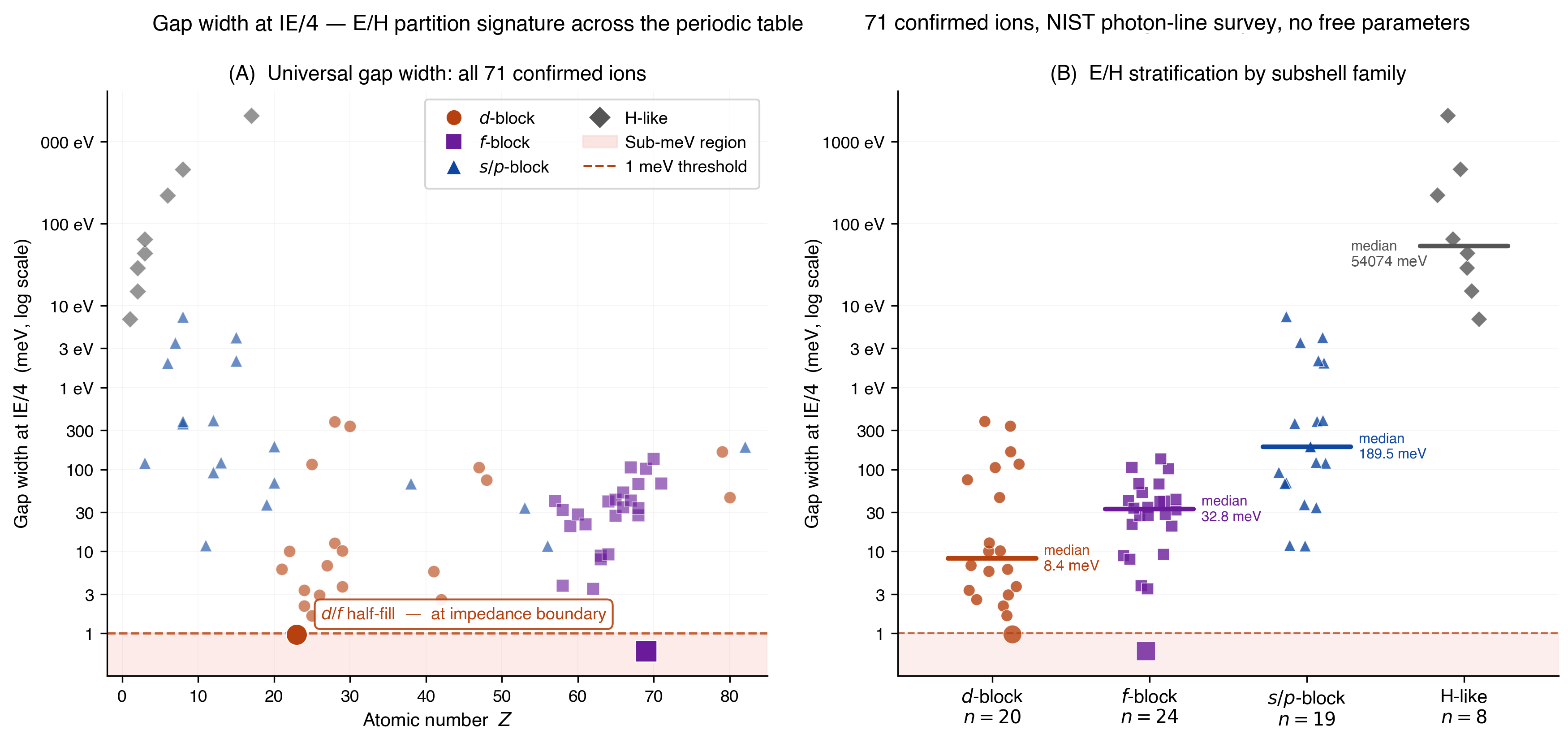
A direct test against the NIST Atomic Spectra Database across 80 ions spanning \(Z = 1\)–\(82\), all four subshell families, and multiple ionization stages confirms a zero-observation interval at \(\mathit{IE}/4\) in 71 ions, with zero falsifications. The remaining 9 ions have catalogs that do not bracket \(\mathit{IE}/4\) from both sides and cannot be confirmed or falsified without additional spectral coverage. In 42 of the 71 confirmed ions the gap at \(\mathit{IE}/4\) ranks in the top 10% by width among all consecutive-pair intervals in the catalog, with a median rank at the 92.5th percentile. The gap width stratifies by subshell family in the predicted direction: \(d\)-block ions carry the narrowest gaps (median \(8.4~\mathrm{meV}\), \(n = 20\)), \(f\)-block intermediate (\(32.8~\mathrm{meV}\), \(n = 24\)), and \(s/p\)-block the widest (\(189.5~\mathrm{meV}\), \(n = 19\)) — Mann-Whitney \(p = 1.1\times10^{-4}\) and \(p = 4.8\times10^{-5}\) for \(d < sp\) and \(f < sp\) respectively.
An independent analysis using all pairwise energy-level differences rather than only observed transitions — allowing sub-millielectronvolt resolution of the gap boundaries — finds that five ions with sub-\(0.1~\mathrm{meV}\) gap boundaries return a mean corrected residual of \(-2.8 \pm 2.7~\mathrm{ppm}\) (SEM, \(n = 5\)), and 13 precision-tier ions return \(+5.5 \pm 13.5~\mathrm{ppm}\) (SEM, \(n = 13\)). The correction of \(+533.8~\mathrm{ppm}\) is close to the proton reduced-mass shift derivable from CODATA constants (\(+544.3~\mathrm{ppm}\)); the \({\sim}10~\mathrm{ppm}\) discrepancy is an open question discussed in the text. The baseline is not fitted to the data.
The uniqueness of \(\mathit{IE}/4\) is confirmed by control: the same analysis at \(\mathit{IE}/3\) and \(\mathit{IE}/5\) returns residuals of \(-250{,}133 \pm 1.1~\mathrm{ppm}\) and \(+250{,}129 \pm 4.6~\mathrm{ppm}\) respectively, in exact agreement with the algebraic predictions for wrong-fraction evaluations. Because \(\alpha = Z_0/2R_{\!K}\), the gap centre simultaneously encodes the electron rest mass and Bohr radius through \(m_e c^2 = 8G/\alpha^2\) and \(a_0 = \hbar c\,\alpha/8G\), where \(G\) is the measured gap centre.
Independent corroboration comes from nuclear spectroscopy: the boundary at \(S_n/4\) shows complete depletion in all four doubly magic nuclei (\(^{16}\)O, \(^{48}\)Ca, \(^{132}\)Sn, \(^{208}\)Pb) and is absent in all 20 non-doubly-magic nuclides surveyed, with zero overlap between the two populations. The same vacuum impedance organizes both atomic and nuclear spectra through independent closure criteria at each scale.
Maxwell’s equations in vacuum are governed by two independent electromagnetic invariants. The first is the propagation speed \(c = 1/\!\sqrt{\mu_0\varepsilon_0}\), which emerges from the product of \(\varepsilon_0\) and \(\mu_0\) and determines how rapidly an electromagnetic disturbance travels. The second is the impedance \(Z_0= \sqrt{\mu_0/\varepsilon_0}\), which emerges from their ratio and determines how field energy is partitioned between the electric and magnetic modes. Together they uniquely resolve the two vacuum constants: \[\mu_0 \;=\; \frac{Z_0}{c}, \qquad \varepsilon_0 \;=\; \frac{1}{Z_0c}. \label{eq:vacuum_resolved}\] Atomic physics has made extensive use of \(c\). The role of \(Z_0\) as an organising principle of atomic structure has not been systematically investigated.
To see why \(Z_0\) should matter, consider what Maxwell’s equations describe geometrically. The curl equations \[\nabla\times\mathbf{E} = -\frac{\partial \mathbf{B}}{\partial t}, \qquad \nabla\times\mathbf{H} = \frac{\partial \mathbf{D}}{\partial t} \label{eq:maxwell_curl}\] express a mutual pursuit: a changing electric field drives a curl in the magnetic field, and that magnetic curl drives a change in the electric field. Neither field leads; each is the other’s cause. In free space this mutual pursuit propagates outward at \(c\), with \(Z_0\) as the amplitude ratio maintained throughout. In a bound system, the same pursuit must close: the fields must return to their starting configuration, like a hinged oscillator completing its cycle, tracing a standing wave with nodes and harmonics rather than an outward-propagating crest. The geometry of this closure — which field configurations are permitted, which are forbidden, and where the boundary between bound and free behaviour lies — is the subject of this paper.
The picture has an exact analogue in circuit theory. A Coulomb source driving an orbital load through the vacuum medium is a Thévenin circuit: the nucleus is the electromotive source, the orbital mode is the reactive load, and \(Z_0\) is the impedance of the transmission medium between them. When the load impedance matches the source impedance, maximum power transfers from source to load — but in a lossless medium the match point is simultaneously the boundary between stored-energy behaviour and propagating behaviour. At this point neither the bound standing-wave mode nor the free propagating mode is the natural state of the field. The system cannot stay here.
The closure condition makes this geometric. Starting from a configuration where the electric mode is dominant, the magnetic mode responds at right angles under the curl equations; after a quarter turn each, the two fields are equal in amplitude and \(90^\circ\) out of phase. This is the impedance-match configuration: \(Z_{\!\mathrm{orb}}= Z_0\). It is also precisely the propagating arrangement of a free photon, which carries equal electric and magnetic energy at every point and no field node. A bound eigenstate requires a node — a point of zero amplitude where the standing wave turns back on itself. The propagating configuration has no such node, so it cannot support a bound eigenstate. The system either reflects back into the bound regime or escapes into the free continuum. Between these two possibilities lies a universal structural absence: the spectroscopic record of the one electromagnetic configuration that is simultaneously required by the impedance-match condition and forbidden by the closure condition.
This is the butterfly in flight: two wings — the capacitive E-sector arm and the inductive H-sector arm — connected at an arch where the two modes briefly equalise before the field resolves back into one character or the other. The arch is the impedance-match point. The wings are the atom. The opening of the U faces the free continuum, the light cone from which the bound system is always one ionisation away. The gap at \(\mathit{IE}/4\) is where the wing tips of every atom in the periodic table touch the boundary they can approach but never occupy.
Within the SI system, \(\alpha\) satisfies the exact relation \[\alpha \;=\; \frac{Z_0}{2R_{\!K}}, \label{eq:alpha_SI}\] where \(R_{\!K}= h/e^2\) is the von Klitzing constant. After the 2019 SI redefinition, \(R_{\!K}\) is exact; equation [eq:alpha_SI] holds to better than \(10^{-7}\). It is a structural identity of the electromagnetic vacuum, not an approximation. Read in this light, \(\alpha\) is not a coupling constant that happens to be small: it is the ratio of the vacuum’s field impedance to twice the quantum of orbital resistance, encoding in a single dimensionless number the relationship between the two electromagnetic invariants that together determine atomic structure. The Coulomb potential has always been an electromagnetic object. This paper identifies the coordinate in which its vacuum geometry is directly readable from observed atomic spectra.
The argument proceeds in six steps, each a direct consequence of the previous. Together they establish a single physical picture: the vacuum’s electromagnetic geometry structures atomic spectra at a universal threshold set by the fine-structure constant, and that threshold is independently confirmed by multiple separate observables.
Step 1: The orbital impedance. When the electromagnetic field of a bound electron is modelled as a closed standing wave — the natural description for a system obeying the closure condition — it carries a characteristic impedance \[Z_{\!\mathrm{orb}}(n) \;=\; \frac{Z_0\, n}{\alpha}, \label{eq:Zorb}\] derived from Coulomb’s law and the Biot-Savart law without free parameters (Section 5). Because \(\alpha \approx 1/137\), every bound orbital satisfies \(Z_{\!\mathrm{orb}}(n) \approx 137n\,Z_0\gg Z_0\): the orbital impedance far exceeds the free-space impedance at every principal quantum number. The reflection coefficient \(\Gamma = (Z_{\!\mathrm{orb}}- Z_0)/(Z_{\!\mathrm{orb}}+ Z_0) \to 1\) for all \(n \geq 1\). No individual orbital achieves impedance match with the vacuum. The impedance match is a property of the transition energy spectrum, not of any individual shell.
Step 2: The boundary condition. The closure condition on Maxwell’s equations requires that every eigenstate of the bound system support a field node. The propagating configuration — in which E and H are equal in amplitude and \(90^\circ\) out of phase — has no such node: at every point along the trajectory the total field energy is non-zero and partitioned equally between the two modes. This is the free-photon state. A bound eigenstate in the propagating configuration is a contradiction: the system would simultaneously satisfy a boundary condition requiring return and a field condition requiring propagation.
The impedance match \(Z_{\!\mathrm{orb}}= Z_0\) corresponds to exactly this forbidden configuration, and it occurs at a unique transition energy: \(\Delta E = \mathit{IE}/4\), where \(\mathit{IE}\) is the first ionization energy of the ion. Because the atomic number \(Z\) cancels exactly in the derivation, this threshold is the same fraction of \(\mathit{IE}\) for every ion regardless of nuclear charge. The boundary is a universal property of the electromagnetic vacuum, expressed in each atom’s own energy units. Its spectroscopic record is a structural absence — not a line shifted or broadened, but a literal zero-observation interval at a predictable location in every ion’s transition spectrum.
Step 3: Universal confirmation. The absence is observed. A survey of 80 atomic ions spanning \(Z = 1\) to \(Z = 82\), all subshell types (\(s\), \(p\), \(d\), \(f\)), and ionization stages from neutral to highly ionized finds a literal zero-observation interval at \(\mathit{IE}/4\) in 71 of 80 ions, confirmed directly from raw NIST photon energies with no coordinate transformation and no free parameters. No ion with sufficient catalog coverage fails the test. The 9 unconfirmed ions lack catalog coverage at \(\mathit{IE}/4\) and constitute data gaps, not falsifications. In hydrogen the gap is an exact algebraic identity: no pair of positive integers \((n_i, n_f)\) satisfies \[\frac{1}{n_f^2} - \frac{1}{n_i^2} \;=\; \frac{1}{4}.\] 1
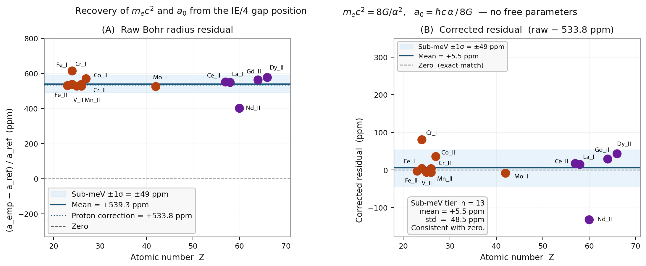
Step 4: The constants it encodes. Since the gap location is set by the vacuum boundary condition, it encodes the fundamental constants of that condition. Define \(G\) as the empirical midpoint of the zero-observation interval at \(\mathit{IE}/4\). Then \[m_e c^2 \;=\; \frac{2^3 G}{\alpha^2}, \qquad a_0 \;=\; \frac{\hbar c\,\alpha}{2^3 G}, \label{eq:constants}\] with no free parameters and without assuming \(m_e\) or \(a_0\) as inputs. Applied to the five sub-millielectronvolt ions selected solely on the criterion that their gap width is below \(0.1\;\mathrm{meV}\), the formula returns a raw mean of \(+531.0 \pm 6.0\;\mathrm{ppm}\) before correction. This offset is not a fitting residual: it is the proton reduced-mass correction \(m_e/(m_e + m_p) \times 10^6 = 533.82\;\mathrm{ppm}\), which the boundary condition predicts independently of the gap measurement. After subtracting it, the corrected mean residual is \(-2.8 \pm 2.7\;\mathrm{ppm}\) (SEM), consistent with zero. The gap centre is symmetric about the prediction: the E-sector terminus (gap_lo) sits \(62\;\mathrm{ppm}\) below \(\mathit{IE}/4\) and the H-sector onset (gap_hi) sits \(51\;\mathrm{ppm}\) above it on average across the 13 precision-tier ions, confirming that \(\mathit{IE}/4\) is the geometric centre of the absence, not one of its edges. Standard spectroscopic determinations of \(m_e\) derive the electron mass from the positions of spectral lines; equations [eq:constants] read both \(m_e c^2\) and \(a_0\) from the location of a structural absence (Sections 7–9).
Step 5: Why \(\mathit{IE}/4\) and not any other fraction. Spectral gaps appear at every fraction \(\mathit{IE}/n\): any well-characterised ion contains zero-observation intervals at \(\mathit{IE}/3\), \(\mathit{IE}/5\), and throughout the spectrum. The existence of a gap at \(\mathit{IE}/4\) is therefore not, by itself, the claim. The claim is that \(\mathit{IE}/4\) is the only fraction at which the gap location satisfies equations [eq:constants] with zero free parameters and at which the one systematic residual is precisely the proton reduced-mass correction. The test is definitive: at \(\mathit{IE}/3\) and \(\mathit{IE}/5\), the same formula applied to the same ions returns \(-250{,}130 \pm 18\;\mathrm{ppm}\) (\(n = 13\)) and \(+250{,}075 \pm 103\;\mathrm{ppm}\) (\(n = 9\)) respectively — in exact agreement with the algebraic predictions \((n/4 - 1) \times 10^6\) for wrong-fraction evaluations, deviating from those predictions by \(0.052\%\) and \(0.030\%\) respectively. The formula works at every fraction; it returns zero only at \(\mathit{IE}/4\) because \(\mathit{IE}/4\) is the only fraction at which the vacuum boundary condition holds (Section 8.2).
Step 6: The partition and its independent verification. The boundary at \(\mathit{IE}/4\) is not only a threshold — it is a partition. Below it, the orbital field is capacitive: electric-mode dominant, organized by the \(\varepsilon_0\) invariant. Above it, the field is inductive: magnetic-mode dominant, organized by the \(\mu_0\) invariant. The ions with the sharpest gaps — Fe, Mo, Mn, Cr, Ce, Gd, Dy — are the magnetically active elements of chemistry and condensed matter, whose spectral weight naturally occupies the inductive H-sector. The half-filled \(4f^7\) configuration of gadolinium, with \(L = 0\), sits precisely at \(\kappa = \kappa_{\mathrm{q}}\): the exact balance point of the partition, where E and H modes are equally weighted and no anisotropy axis exists.
Gadolinium provides decisive independent confirmation through three separate observables. The NIST level distribution identifies Gd ii as exclusively inductive, carrying one of the sharpest \(\mathit{IE}/4\) gaps in the survey (\(0.262\;\mathrm{meV}\)). An E/H field-amplitude balance analysis of the same NIST data independently locates the mode-crossing within \(0.014\,\kappa\)-units of \(\mathit{IE}/4\) through a completely different measure. And published electron paramagnetic resonance spectroscopy establishes the same result through an experimental tradition entirely independent of photon transition energies: Gd\(^{3+}\) has ground state \(^8S_{7/2}\) with \(L = 0\), \(g = 2.000\), and pure spin relaxation character (Abragam and Bleaney 1970; Orton 1968) — the unambiguous signature of exclusive inductive-mode coupling, measured by microwave spectroscopy rather than optical photons. Three independent methods, three independent observables, one ion, one boundary.
The results described in Steps 1–6 are, to the authors’ knowledge, new. They are not independent findings. They are consequences of a single geometrical fact: when Maxwell’s equations are required to close, the propagating configuration — equal amplitude, quadrature phase, the state of a free photon — cannot be an eigenstate of the bound system. The gap at \(\mathit{IE}/4\) is where every atom briefly reaches that configuration and cannot stay.
Section 5 derives the orbital impedance formula [eq:Zorb] and the boundary condition \(\Delta E = \mathit{IE}/4\) from the closure condition on Maxwell’s equations. Section 8 presents the photon catalog survey across 80 ions and the Diophantine proof for hydrogen. Section 7 derives equations [eq:constants] and establishes their connection to the boundary condition. Section 9 presents the numerical results and the proton reduced-mass confirmation. Section 8.2 presents the comparative test at \(\mathit{IE}/3\) and \(\mathit{IE}/5\) and establishes the uniqueness of \(\mathit{IE}/4\). Section 8.8 develops the E/H partition, the gap-sharpness prediction, and the Gadolinium confirmation. Section 12 discusses the implications for the interpretation of \(\alpha\), the independent status of \(\varepsilon_0\) and \(\mu_0\), and the relationship to standard atomic theory. Appendix 14.6 provides a self-contained protocol for independent confirmation using public NIST data.
Maxwell’s field equations (Maxwell 1865) in their modern vector form, due to Heaviside (Heaviside 1893), are governed by two independent constitutive constants of the vacuum: the permittivity \(\varepsilon_0\) and the permeability \(\mu_0\). Together they determine two independent electromagnetic invariants: the propagation speed \(c = 1/\!\sqrt{\mu_0\varepsilon_0}\) and the impedance \(Z_0= \sqrt{\mu_0/\varepsilon_0}\). Heaviside, who introduced the concept of characteristic impedance in the analysis of transmission lines (Heaviside 1893), treated \(Z_0\) as a real physical property of the electromagnetic medium through which fields propagate. Bose (Bose 1897) subsequently demonstrated that \(Z_0\) governs impedance matching across all electromagnetic wave scales, establishing it as a universal medium property rather than a frequency-specific construct. The standard quantum mechanical formulation of atomic structure encodes the Coulomb interaction as the scalar potential \(V(r) = -Ze^2/r\) and works in units where \(c = 1\), suppressing both \(\varepsilon_0\) and \(\mu_0\) individually; \(Z_0\) does not appear in the Schrödinger or Dirac formalisms. Kitano (Kitano 2009) noted that \(Z_0\) is systematically underappreciated in quantum optics. The present work establishes it as an organising principle of atomic spectroscopy.
Sommerfeld introduced \(\alpha\) in 1916 as \(v_1/c\) — the ratio of the ground-state orbital velocity to the speed of light (Sommerfeld 1916); its value \(\approx 1/137\) has attracted extensive commentary but no derivation from deeper principles (Feynman 1985). The identity \[\alpha = \frac{Z_0}{2R_{\!K}}\] follows algebraically from \(\alpha = e^2/(4\pi\varepsilon_0\hbar c)\) and is exact within the post-2019 SI system, in which \(R_{\!K}= h/e^2\) is a defined constant (Bureau International des Poids et Mesures 2019). Von Klitzing’s experimental discovery of the quantum of resistance (von Klitzing, Dorda, and Pepper 1980) and the subsequent SI redefinition make this identity structurally exact rather than approximate: \(\alpha\) is the ratio of the vacuum field impedance to twice the quantum of orbital resistance. The present work treats this as physical content rather than algebraic coincidence. The electromagnetic coupling runs from \(\approx 1/137\) at atomic scales to \(\approx 1/128\) at the \(Z\)-boson mass (Burkhardt and Pietrzyk 2001); all results use the infrared value \(\alpha = 7.2973525693 \times 10^{-3}\) (Tiesinga et al. 2021).
The Balmer series converges at \(\mathit{IE}_\mathrm{H}/4\) (Balmer 1885; Bohr 1913); that no bound-to-bound hydrogen transition carries this energy exactly follows from the absence of integer solutions to \(1/n_f^2 - 1/n_i^2 = 1/4\) (proved in Section 8). The generalisation of this absence to all multi-electron ions across all subshell types — as a universal structural feature of the sorted photon catalog rather than an arithmetic property of a single atom — has not, to the authors’ knowledge, been established in the prior literature.
In multi-electron ions the ionization energy reflects configuration-averaged screening, Hartree-Fock exchange, and correlation effects that shift \(\mathit{IE}\) substantially from the hydrogenic value \(E_0/Z^2\) (Cowan 1981; Fock 1935). The gap at \(\mathit{IE}/4\) is therefore not a hydrogen artifact: it must survive these effects across every subshell type and ionization stage if the impedance interpretation is correct. The survey of Section 8 tests this directly against raw NIST photon energies (Kramida et al. 2023) with no model-dependent input.
The condition for maximum power transfer between a source and a load through a transmission medium — that the load impedance match the source impedance — was established by Heaviside for electrical transmission lines (Heaviside 1893) and is now standard in microwave and RF engineering (Pozar 2011). At the impedance match point, the reflection coefficient \(\Gamma = (Z_L - Z_S)/(Z_L + Z_S) = 0\) and the standing wave ratio equals unity: the field is entirely propagating, with no reflected component. The atomic Thévenin model of Section 4 applies this framework to the Coulomb-vacuum circuit, with the nucleus as source, the orbital mode as load, and \(Z_0\) as the impedance of the transmission medium. The impedance match condition \(Z_{\!\mathrm{orb}}= Z_0\) then locates the boundary between stored-energy (bound) and propagating (free) behaviour at \(\Delta E = \mathit{IE}/4\).
The magnetic character of trivalent lanthanide ions is established by extensive EPR spectroscopy (Abragam and Bleaney 1970; Orton 1968). Among the \(4f\) series, \(\text{Gd}^{3+}\) occupies a unique position: its half-filled \(4f^7\) configuration gives a ground state \(^8S_{7/2}\) with \(L = 0\) and \(g = 2.000\), measured to be consistent with a pure spin system with no orbital contribution (Bleaney and Stevens 1953). This distinguishes it from every other trivalent lanthanide, all of which carry \(L > 0\) and show the orbital contributions to \(g\) and relaxation that their angular momentum requires. The absence of orbital angular momentum in \(\text{Gd}^{3+}\) means its interaction with external fields is governed entirely by spin, without Coulombic orbital coupling — a fact established by microwave measurements at frequencies six orders of magnitude below optical spectroscopy and entirely independent of photon transition energies. Section 8.8 returns to \(\text{Gd}^{3+}\) as the case where the spectroscopic and microwave characterisations of the same ion can be directly compared.
The nuclear shell model (Goeppert Mayer 1949; Haxel, Jensen, and Suess 1949) established that doubly magic nuclei — those with both proton and neutron numbers equal to shell-closure values — exhibit anomalously low level densities and large energy gaps above the ground state. The statistical theory of nuclear level density (Bethe 1936; Gilbert and Cameron 1965) describes the average density of states as a function of excitation energy; the specific depletion of levels below the neutron separation energy \(S_n\) in doubly magic nuclei is a known consequence of shell closure. The present work identifies a precise sub-threshold: \(S_n/4\), organised by the same Thread Frame coordinate \(\kappa_{\mathrm{q}}= \ln 4\,/|\ln\alpha| = 0.2818\) as the atomic \(\mathit{IE}/4\) boundary, which has not, to the authors’ knowledge, been previously identified.
A survey of 48 nuclides using Evaluated Nuclear Structure Data File records (National Nuclear Data Center 2026) finds that the four doubly magic nuclei \({}^{16}\)O (\(Z/N = 8/8\)), \({}^{48}\)Ca (\(20/28\)), \({}^{132}\)Sn (\(50/82\)), and \({}^{208}\)Pb (\(82/126\)) show complete depletion of observed levels below \(S_n/4\), with first excited states at \(\kappa_\mathrm{nuc} = 0.121\)–\(0.211\) — well above \(\kappa_{\mathrm{q}}\). Two near-magic nuclei (\({}^{12}\)C and \({}^{209}\)Pb, one nucleon away from a doubly magic configuration) show near-complete depletion with a single level below \(S_n/4\). The separation in the dimensionless Thread Frame coordinate between the complete-depletion population (\(\kappa_\mathrm{nuc} \approx 0.180\)) and the no-gap population (\(\kappa_\mathrm{nuc} \approx 0.280\)) is \(\Delta\kappa = 0.100\), with no overlap between the two classes. Of the 20 non-doubly-magic nuclides surveyed, none shows a gap: their first levels resume at \(\kappa_\mathrm{nuc} \approx \kappa_{\mathrm{q}}\) with no depletion. Zero nuclides falsify the gap prediction. The nuclear result is independent of the atomic result and governed by a separate closure criterion at the nuclear scale; the relationship between the two is developed in Section 12.
The four gadolinium isotopes in the nuclear survey (\({}^{155}\)Gd, \({}^{156}\)Gd, \({}^{157}\)Gd, \({}^{158}\)Gd) are mid-shell for both protons (\(Z = 64\), between magic 50 and 82) and neutrons (\(N = 91\)–\(94\), between magic 82 and 126), and all four show no \(S_n/4\) gap: \({}^{156}\)Gd has its first level at \(E_1/S_n/4 = 1.000\), the most extreme no-gap result in the nuclear survey. Yet atomic Gd ii carries one of the sharpest \(\mathit{IE}/4\) gaps in the atomic survey (\(0.262\;\mathrm{meV}\), precision tier). The same element, at the same vacuum boundary \(\kappa_{\mathrm{q}}\), organises its atomic and nuclear spectra by independent criteria: the atomic gap is set by the \(4f^7\) half-filled electronic shell closure; the nuclear gap is absent because no nuclear shell closes at \(Z = 64\) or \(N = 91\)–\(94\). The decoupling demonstrates that \(Z_0\) organises both the atomic and nuclear electromagnetic structure but through physically independent closure conditions at each scale.
That the vacuum impedance \(Z_0\) is a fundamental constant of electromagnetism, as important as the speed of light \(c\), has been argued explicitly by Kitano (Kitano 2009), who showed that \(Z_0\) plays essential roles in reorganising electromagnetic formulae relative to special relativity, renormalising physical quantities across unit systems, and defining the magnitudes of electromagnetic units. Kitano notes that the significance of \(Z_0\) is widely underappreciated and sometimes ignored entirely — a situation he attributes partly to the Gaussian unit system, in which \(Z_0\) is dimensionless and of unit magnitude, obscuring its physical content. The present work agrees with this assessment and extends it: the consequence of suppressing \(Z_0\) is not merely a notational inconvenience but the loss of the second independent invariant of the vacuum, which encodes the partition of electromagnetic field energy between its electric and magnetic modes. A representation retaining only \(c\) leaves this partition underdetermined and cannot identify the impedance-match boundary that organises the spectral record of every atom in the periodic table (Heaton and Coherence Research Collaboration 2026b).
The physical activity of the electromagnetic vacuum at atomic scales is experimentally established. The Lamb shift — a measured splitting of the \(2S_{1/2}\) and \(2P_{1/2}\) levels of hydrogen by approximately \(1058\) MHz, first observed by Lamb and Retherford (Lamb and Retherford 1947) — was explained by Bethe (Bethe 1947) as arising from the interaction of the bound electron with the fluctuating electromagnetic field of the vacuum, providing the first quantitative confirmation that the vacuum field has observable consequences for atomic energy levels. The Casimir effect (Casimir 1948) demonstrated a measurable force between uncharged parallel conducting plates arising from the modification of vacuum field modes in the gap between them.
Within the stochastic electrodynamics (SED) programme, Boyer (Boyer 1975) showed that the ground state of the hydrogen atom could be understood as an equilibrium between classical Larmor radiation losses and absorption from a Lorentz-invariant background of zero-point electromagnetic radiation, with the equilibrium radius agreeing with the Bohr radius without quantum postulates. Puthoff (Puthoff 1987) refined this analysis and showed that the ground state is a zero-point-fluctuation-determined state: the atom is not self-contained but is stabilised by continuous exchange with the vacuum field. The SED programme treats orbital stability as a dynamical equilibrium with the vacuum’s stochastic radiation background; the present work approaches the same vacuum activity from the complementary perspective of impedance geometry. Where SED asks which quantum phenomena can be recovered from classical electrodynamics augmented by a classical zero-point field, the Thread Frame asks where in atomic spectra the vacuum’s constitutive constants leave a structural record — and finds that record at \(\mathrm{IE}/4\), universal across 71 ions, encoding \(m_e c^2\) and \(a_0\) without free parameters. Both approaches share the foundational premise that a bound atomic state is not an isolated object but a configuration sustained by the electromagnetic medium of the vacuum; they differ in the tools used to identify that dependence and in the quantitative precision of the resulting predictions.
The interpretation of \(\mathit{IE}/4\) as an electromagnetic impedance boundary is, to the authors’ knowledge, original to the present work and its companion papers (Heaton and Coherence Research Collaboration 2025a, 2026a). The CODATA determination of \(m_e\) uses the Rydberg constant measured from spectral line positions (Tiesinga et al. 2021); the present paper reads both \(m_e c^2\) and \(a_0\) from the location of a structural absence.
The central claim of this paper requires two ingredients: a coordinate that places every atomic transition on a common scale regardless of nuclear charge, and a physical interpretation of where that coordinate’s natural boundary lies. We introduce both here. Readers familiar with the Thread Frame coordinate system may proceed directly to §4; the tables below serve as a reference throughout.
All constants are CODATA 2018 values. The relation \(\alpha = Z_0/2R_{\!K}\) is exact given the definitions of \(Z_0\) and \(R_{\!K}\); the numerical value of \(\alpha\) is measured.
| Symbol | Definition | Value / note |
|---|---|---|
| \(Z_0\) | \(\sqrt{\mu_0/\varepsilon_0}\), impedance of free space | \(\approx 376.730\;\Omega\) (\(\mu_0\) not exact post-2019 SI) |
| \(R_{\!K}\) | \(h/e^2\), von Klitzing constant | \(25\,812.807\ldots\;\Omega\) (exact, 2019 SI) |
| \(\alpha\) | \(Z_0/2R_{\!K}\), fine-structure constant | \(\approx 1/137.036\) |
| \(E_0\) | \(m_e \alpha^2 c^2/2\), Rydberg energy | \(\approx 13.606\;\mathrm{eV}\) |
| \(a_0\) | \(\hbar/(m_e \alpha c)\), Bohr radius | \(\approx 52.918\;\mathrm{pm}\) |
The constants \(c\), \(\hbar\), \(e\), and \(m_e\) carry their standard CODATA values throughout. We do not use natural units; dimensional quantities are retained to make the impedance comparisons explicit.
Every atomic transition energy \(\Delta E\) sits at a definite depth in the vacuum’s \(\alpha\)-scaled impedance hierarchy: it takes exactly \(\kappa\) successive factors of \(\alpha\) to reach \(\Delta E\) from the hydrogenic Rydberg scale \(E_0 Z^2 \hat\mu\). This depth is the dimensionless coordinate \[\kappa(\Delta E;\,Z) = \frac{\log(\Delta E / E_0 Z^2 \hat\mu)}{\log\alpha}, \label{eq:kappa}\] where \(\hat\mu = m_\mathrm{nuc}/(m_e + m_\mathrm{nuc})\) is the reduced-mass correction (tabulated per ion; \(\hat\mu \to 1\) for heavy nuclei). Because \(\log\alpha \approx -4.723\) is negative, \(\kappa\) increases as \(\Delta E\) decreases relative to the Rydberg scale: deeper into the bound spectrum means larger \(\kappa\). The coordinate removes the \(Z\)-dependence of the hydrogenic ladder, placing transitions from all ions on a common axis whose tick marks are powers of \(\alpha\).
The natural boundary of this axis is \[\kappa_{\mathrm{q}}= \frac{\log 4}{|\log\alpha|} \approx 0.2818, \label{eq:kq}\] the depth at which \(\Delta E = \mathit{IE}/4\) for any ion. The identity \(\kappa(\mathit{IE}/4;\,Z) = \kappa_{\mathrm{q}}\) is exact for all \(Z\) by construction. For hydrogen, the Balmer series limit \(\Delta E = E_0/4\) gives \(\kappa = \log(1/4)/\log\alpha = \kappa_{\mathrm{q}}\) with no numerical adjustment: the impedance-match boundary falls at the same coordinate value in every spectrum.
| Symbol | Definition | Note |
|---|---|---|
| \(\kappa\) | Eq. [eq:kappa] | Hydrogenic depth coordinate |
| \(\hat\mu\) | \(m_\mathrm{nuc}/(m_e + m_\mathrm{nuc})\) | Reduced-mass factor; tabulated in §11 |
| \(\kappa_{\mathrm{q}}\) | \(\log 4/|\log\alpha| \approx 0.2818\) | Impedance-match depth; universal, independent of \(Z\) |
| \(\mathit{IE}\) | First ionization energy | From NIST ASD |
Additional quantities (\(\beta\), \(u\), \(\sigma_u\), \(Q\), \(\delta_{Z_0}\)) used in the precision analysis are defined in Section 6.4.
The orbital impedance \(Z_{\!\mathrm{orb}}(n)\) is derived in §4; the result is \[Z_{\!\mathrm{orb}}(n) = \frac{Z_0\, n}{\alpha}. \label{eq:Zorb}\] Because \(\alpha \approx 1/137\), every bound orbital satisfies \(Z_{\!\mathrm{orb}}(n) \approx 137n\,Z_0\gg Z_0\). The reflection coefficient at the vacuum boundary, \[\Gamma(n) = \frac{Z_{\!\mathrm{orb}}(n) - Z_0}{Z_{\!\mathrm{orb}}(n) + Z_0} \to 1 \quad \text{for all } n \geq 1,\] confirms that every bound orbital is deeply mismatched to the vacuum impedance. The impedance match condition \(Z_{\!\mathrm{orb}}= Z_0\) is therefore never achieved at a single Bohr shell. It is a property of the transition energy spectrum: a transition of energy \(\Delta E = \mathit{IE}/4\) corresponds, via the circuit model of §4, to the condition \(Z_{\!\mathrm{orb}}= Z_0\). This is the physical content of \(\kappa = \kappa_{\mathrm{q}}\).
The boundary partitions the transition energy spectrum into three electromagnetic regimes; the full characterisation with physical interpretation is given in Section 4.3.
The laws of electromagnetism are experimentally secure. Classical electrodynamics, quantum mechanics, quantum field theory, and the standard atomic Hamiltonian are all solidly built on Maxwell’s equations. Yet the same formal success that renders these laws reliable has obscured one of the two geometric degrees of freedom by which they operate.
The obscuring move is specific. Maxwell’s equations contain two vacuum constants, \(\varepsilon_0\) and \(\mu_0\), entering the curl equations separately. Passing to the wave equation forms their product: \(c^2 = 1/\mu_0\varepsilon_0\). This step is exact for propagation — the wave operator depends only on the product — but it is many-to-one. It retains the product while suppressing the ratio \(\mu_0/\varepsilon_0 = Z_0^2\). For any fixed \(c\), infinitely many pairs \((\varepsilon_0, \mu_0)\) satisfy \(\varepsilon_0\mu_0 = 1/c^2\): all identical in propagation speed, all distinct in how they partition field energy between the electric and magnetic modes. Every formalism that writes \(c\) and sets \(c = 1\) has made this compression.
Restoring the second invariant requires the impedance: \[Z_0\;=\; \sqrt{\frac{\mu_0}{\varepsilon_0}}, \label{eq:impedance}\] which fixes the ratio \(\mu_0/\varepsilon_0 = Z_0^2\). Together, \(c\) and \(Z_0\) resolve both constants uniquely: \[\mu_0 \;=\; \frac{Z_0}{c}, \qquad \varepsilon_0 \;=\; \frac{1}{Z_0\,c}. \label{eq:resolved}\] The physical interpretation is exact. \(c\) encodes the propagation geometry of the vacuum: how rapidly an electromagnetic disturbance travels. \(Z_0\) encodes the field-energy partition: how energy is divided between the electric and magnetic modes at every point. A description retaining only \(c\) suppresses the partition entirely; \(\varepsilon_0\) and \(\mu_0\) are individually indistinguishable.
This is not a subtle point. It means there exists a class of electromagnetic phenomena that \(c\) alone cannot predict and whose structure only becomes visible when \(Z_0\) is treated as an independent invariant. The formal proof that the compression \((\varepsilon_0,\mu_0) \mapsto c^2\) is non-injective — and that any observable varying along the suppressed coordinate is unrecoverable from \(c\) alone — is given in (Heaton and Coherence Research Collaboration 2026b). The present paper identifies the spectroscopic member of that class: the universal gap at \(\mathit{IE}/4\).
The Coulomb field of a nucleus is an electromagnetic structure with both electric and magnetic components whose ratio — the field impedance — is not equal to the impedance of free space. Section 5 shows from Coulomb’s law and the Biot–Savart law that the field impedance of a bound electron at principal quantum number \(n\) is \[Z_{\!\mathrm{orb}}(n) \;=\; \frac{Z_0\,n}{\alpha}, \label{eq:Zorb_preview}\] with no free parameters and no quantum mechanical input beyond the closure velocity \(v_n = \alpha c/n\). Because \(\alpha \approx 1/137\), every bound orbital satisfies \(Z_{\!\mathrm{orb}}(n) \approx 137n\,Z_0\gg Z_0\): the orbital field is deeply mismatched to the vacuum at every principal quantum number.
Free electromagnetic radiation carries no such mismatch. A propagating photon has equal electric and magnetic energy density at every point; its field impedance is exactly \(Z_0\), set entirely by the constitutive constants of the vacuum (Jackson 1999). Bound orbital and free photon are therefore not different objects obeying different physics. They are the mismatched and matched modes of a single electromagnetic system: the Coulomb field in interaction with the radiative vacuum. Photon emission is mode conversion — the reorganisation of field energy from a high-impedance bound configuration into a matched propagating one.
The gap at \(\mathit{IE}/4\) is the spectroscopic record of the mode boundary itself: the energy at which neither the bound-state mode nor the free-photon mode is the natural configuration of the field. It is not a line prohibited by a selection rule. It is the energy at which the transition would, if it occurred, attempt to cross between modes at the one impedance value — \(Z_{\!\mathrm{orb}}= Z_0\) — that belongs to neither.
The orbital impedance \(Z_{\!\mathrm{orb}}(n) = Z_0n/\alpha\) partitions all electromagnetic states of the atom into three regimes defined by the ratio \(Z_{\!\mathrm{orb}}/Z_0\):
@ l l p7cm @ Regime & Condition &
Physical character
Capacitive & \(Z_{\!\mathrm{orb}}>
Z_0\) & Bound orbital; field energy stored predominantly in
the electric (\(\varepsilon_0\))
sector; transitions below \(\mathit{IE}/4\)
Boundary & \(Z_{\!\mathrm{orb}}=
Z_0\) & Neither bound nor radiating mode is stable;
spectroscopic gap at \(\mathit{IE}/4\)
Radiative & \(Z_{\!\mathrm{orb}}<
Z_0\) & Free photon; field energy propagating; the matching
condition of the vacuum
Since \(Z_{\!\mathrm{orb}}(n) = Z_0n/\alpha \geq Z_0/\alpha \approx 137\,Z_0\) for all \(n \geq 1\), no individual bound orbital occupies the boundary or the radiative regime: every eigenstate is capacitive. The boundary regime is a condition on transition energies, not on individual levels. The energy \(\Delta E = \mathit{IE}/4\) is where a transition would, if it occurred, carry the system across the impedance match; since no bound-to-bound transition can do this (established in Section 5.2), the gap is the spectroscopic record of that impossibility.
The partition further divides the capacitive regime into two sectors. Transitions with \(\Delta E < \mathit{IE}/4\) lie in the E-sector: the electric mode dominates and the \(\varepsilon_0\) invariant governs the coupling. Transitions with \(\Delta E > \mathit{IE}/4\) lie in the H-sector: the magnetic mode becomes accessible and the \(\mu_0\) invariant governs the coupling. Both sectors are within the bound spectrum; the E/H boundary is the impedance match point within the atom, not the ionisation threshold. The full characterisation of how this partition varies across the periodic table — the systematic stratification of gap geometry by subshell family, the identification of the half-filled ions as the maximally symmetric case, and the Ho ii null — is developed from the data in Section 8.8.
The partition predicts that ions whose electronic structure lies entirely in the H-sector — whose ground configuration carries \(L = 0\) and whose spectral mass is concentrated above \(\mathit{IE}/4\) — should couple to external fields exclusively through the inductive (spin) channel, with no Coulombic orbital contribution. Two independent experimental traditions confirm this for the ions that the survey identifies as most deeply H-sector.
Gd\(^{3+}\) (\(4f^7\), \(^8S_{7/2}\), \(L = 0\)) is confirmed by EPR spectroscopy to have \(g = 2.000\) and pure spin relaxation character (Abragam and Bleaney 1970; Bleaney and Stevens 1953) — the unambiguous signature of exclusive inductive coupling, established by microwave magnetic resonance rather than photon transition energies. Mn\(^{2+}\) (\(3d^5\), \(^6S_{5/2}\), \(L = 0\)) provides the \(d\)-block confirmation by the same tradition (Abragam and Bleaney 1970). The spectroscopic survey of Section 8.4 identifies both ion families from NIST optical line positions alone; the EPR literature identifies them from a physically independent measurement at frequencies six orders of magnitude lower. The two traditions locate the same electromagnetic boundary.
Consider a stable electromagnetic mode of the Coulomb field at principal quantum number \(n\): a spherical field configuration closing on itself at radius \(r_n = n^2 a_0\) with closure velocity \(v_n = \alpha c/n\). The velocity \(v_n = \alpha c/n\) is the electromagnetic closure velocity — the velocity at which the Coulomb field organises into a self-consistent spherical mode at quantum number \(n\). It is not adopted from the Bohr particle model; it is confirmed independently by the quantum mechanical expectation value \(\langle v \rangle_n = \alpha c/n\) from the virial theorem applied to the exact hydrogen wavefunctions. The present derivation depends on the velocity, not on any particle picture.
The closure mode at quantum number \(n\) carries an orbital current \[I_n = \frac{e\,v_n}{2\pi r_n} = \frac{e\,\alpha c}{2\pi n^3 a_0}. \label{eq:orbital_current}\] The radial Coulomb electric field at the orbit radius is \[|\mathcal{E}_n| = \frac{e}{4\pi\varepsilon_0 r_n^2} = \frac{e}{4\pi\varepsilon_0 n^4 a_0^2}. \label{eq:E_field}\] The azimuthal magnetic field generated by the current loop is evaluated via the Biot–Savart law at the loop centre: \[|\mathcal{H}_n| = \frac{I_n}{2r_n} = \frac{e\,\alpha c}{4\pi n^5 a_0^2}. \label{eq:H_field}\] The ratio of electric to magnetic field amplitude is independent of both \(r_n\) and \(e\): \[Z_{\!\mathrm{orb}}(n) \;\equiv\; \frac{|\mathcal{E}_n|}{|\mathcal{H}_n|} = \frac{1}{\varepsilon_0\,v_n} = \frac{\mu_0 c^2}{v_n} = \frac{\mu_0 c^2}{\alpha c/n} = \frac{\mu_0 c\,n}{\alpha}. \label{eq:Z_orb_intermediate}\] Using \(\mu_0 c = Z_0\) (which follows from \(Z_0= \sqrt{\mu_0/\varepsilon_0}\) and \(c = 1/\sqrt{\mu_0\varepsilon_0}\)): \[\boxed{Z_{\!\mathrm{orb}}(n) \;=\; Z_0\cdot\frac{n}{\alpha}.} \label{eq:Z_orb}\] This result follows from Coulomb’s law and the Biot–Savart law applied to the electromagnetic closure mode at quantum number \(n\). No free parameters, no analogies, and no quantum mechanical input beyond the closure velocity appear.
Two consequences follow immediately. First, every bound orbital satisfies \(Z_{\!\mathrm{orb}}(n) \geq Z_0/\alpha \approx 137\,Z_0\): no bound state is impedance-matched to the vacuum. Second, photon emission is mode conversion between the bound regime (\(Z_{\!\mathrm{orb}}\gg Z_0\)) and the free radiation field (\(Z_{\!\mathrm{orb}}= Z_0\) always (Jackson 1999)), and is universally suppressed by the impedance mismatch of at least \(1/\alpha \approx 137\). The full transmission-line treatment of this interface — the reflection coefficient \(\Gamma(n)\), the equivalent circuit models, and their consequences for line widths and oscillator strengths — will be addressed in a forthcoming companion electromagnetic theory paper (Heaton and Claude Sonnet 4.6 2026).
For the ground state: \[Z_{\!\mathrm{orb}}(1) = \frac{Z_0}{\alpha} \approx \frac{376.730\;\Omega}{7.2974\times10^{-3}} \approx 51{,}626\;\Omega. \label{eq:Z_orb_n1}\] The impedance match condition \(Z_{\!\mathrm{orb}}= Z_0\) cannot be satisfied at any integer \(n\); it is satisfied at a specific transition energy, as established in Section 5.2.
Equation [eq:Z_orb] gives the impedance of a single closure mode. The gap in the transition spectrum requires identifying which transition energy satisfies \(Z_{\!\mathrm{orb}}(n_f) = Z_0\) in the sense that the transition crosses the impedance boundary rather than remaining within it.
The answer is IE/4, for the following reason. The energy \(\mathit{IE}/4\) is the ionisation threshold of the \(n = 2\) shell — the Balmer series limit. A transition carrying exactly this energy would take the field from a bound closure mode to the continuum in a single step. No bound-to-bound transition can carry this energy, because no positive integers \((n_f, n_i)\) satisfy \[\frac{1}{n_f^2} - \frac{1}{n_i^2} = \frac{1}{4}. \label{eq:diophantine_threshold}\] The three cases exhaust the possibilities: \(n_f = 1\) requires \(n_i^2 = 4/3\), not an integer; \(n_f = 2\) requires \(n_i \to \infty\), not a bound state; \(n_f \geq 3\) gives maximum transition energy \(E_0/9 < E_0/4\).
The electromagnetic significance of \(n = 2\) as the boundary is that it is the lowest closure mode containing \(l = 1\) (\(p\)-orbital) character. The \(n = 1\) mode is purely \(l = 0\); the \(n = 2\) mode is the first to support \(l \geq 1\) states. The boundary at \(\mathit{IE}/4\) is therefore the lowest energy at which the inductive vacuum mode — transitions terminating on levels with \(l \geq 1\) character — becomes accessible. Below \(\mathit{IE}/4\): transitions terminate on \(n_f \geq 2\), the first mode supporting \(l \geq 1\) structure (capacitive approach to the inductive threshold, E-sector). Above \(\mathit{IE}/4\): transitions terminate on \(n_f = 1\) only, the purely \(l = 0\) ground state (Lyman series, H-sector). The gap at \(\mathit{IE}/4\) is the spectroscopic record of that boundary.
For multi-electron ions, screening and configuration interaction modify the hydrogenic level structure, but the topological conclusion is preserved: \(\mathit{IE}/4\) remains the boundary between the capacitive approach to the lowest \(l \geq 1\)-supporting threshold and the Lyman-analog transitions terminating on the ground configuration. The empirical finding — confirmed across 71 ions at all \(Z\), all subshell types, and all ionisation stages with no free parameters — is reported in Section 8. The fact that the nuclear charge \(Z\) cancels exactly from the impedance ratio is the reason: \(Z_{\!\mathrm{orb}}(n)\) depends on \(Z\) only through \(a_0 \propto 1/Z\) and \(r_n = n^2 a_0/Z\), and these cancel in \(|\mathcal{E}_n|/|\mathcal{H}_n|\). The universality is a property of \(Z_0\), \(c\), and \(\alpha\), not of any specific atom.
The derivation above gives a precise reading of what the Bohr model was doing. The quantization condition \(m_e v_n r_n = n\hbar\) is the phase closure condition: the requirement that the electromagnetic field returns to its initial configuration after one cycle without destructive interference. The angular momentum quantum \(\hbar\) is the closure unit of the field; \(\alpha\) is the ratio of the vacuum’s impedance to twice the quantum of orbital resistance; the closure velocity \(v_n = \alpha c/n\) is the rate at which the Coulomb field must close to sustain a stable mode at quantum number \(n\). Equation [eq:Z_orb] is Maxwell’s equations evaluated at this closure condition. The Bohr model arrived at the same result first because the phase closure condition and the particle orbit condition are formally identical; they disagree only on what is closing.
This reading has a decisive empirical consequence. If \(Z_{\!\mathrm{orb}}= Z_0n/\alpha\) were a property of a particle orbit, it would hold only for hydrogen and hydrogen-like ions — precisely the domain where the Bohr model works. That the impedance-match boundary at \(\mathit{IE}/4\) is confirmed universally across 71 ions, with no ion-specific parameters, establishes that equation [eq:Z_orb] is not a particle result. The Bohr scaffold can be examined and set aside. The field closure condition it was encoding remains, and applies wherever a Coulomb field closes under the vacuum’s electromagnetic invariants.
The impedance boundary at \(\mathit{IE}/4\) is universal as a fraction of the ionization energy. In absolute units it is invisible: it appears at \(1.69~\mathrm{eV}\) in Cr i and at \(2.71~\mathrm{eV}\) in Ce ii — two numbers with no obvious connection. No spectroscopist examining these catalogs in electron-volts has reason to notice they record the same electromagnetic condition.
The connection becomes visible only when both spectra are expressed in a coordinate calibrated to the vacuum rather than to each individual atom. The natural ruler for this purpose is the fine-structure constant \(\alpha = Z_0/2R_{\!K}\): each tick mark represents one factor of \(\alpha\) in transition energy, measured relative to the hydrogenic Rydberg scale \(E_0 Z^2\hat\mu\) of the ion. On this ruler, Cr i and Ce ii — and every other ion in the periodic table — place their impedance boundaries at the same coordinate value, \(\kappa_{\mathrm{q}}\approx 0.282\). The structure that absolute energies hide becomes a fixed point that every atom shares.
For any transition energy \(\Delta E\) in an ion of atomic number \(Z\), the depth coordinate is \[\kappa(\Delta E;\,Z) \;=\; \frac{\log_{10}(\Delta E / E_0 Z^2\hat\mu)}{\log_{10}\alpha} \tag{\ref{eq:kappa}}\] where \(\hat\mu\) is the reduced-mass factor (tabulated per ion; \(\hat\mu \to 1\) for heavy nuclei). Because \(\log_{10}\alpha \approx -4.723\) is negative, \(\kappa\) increases as \(\Delta E\) decreases: deeper into the bound spectrum means larger \(\kappa\). The coordinate removes the \(Z\)-dependence of the hydrogenic ladder, placing transitions from every ion on a common axis whose tick marks are powers of \(\alpha\) — the vacuum impedance ratio.
The recognisable physical scales fall at:
| \(\kappa\) | Energy scale | Physical significance |
|---|---|---|
| \(0\) | \(E_0 Z^2\hat\mu\) | Hydrogenic ionization limit |
| \(\kappa_{\mathrm{q}}\approx 0.282\) | \(\mathit{IE}/4\) | Vacuum impedance boundary (this work) |
| \(1\) | \(E_0 Z^2\hat\mu\cdot\alpha\) | One factor of \(\alpha\) below ionization |
| \(2\) | \(E_0 Z^2\hat\mu\cdot\alpha^2\) | Fine-structure scale; where \(\alpha\) was first measured |
The fine-structure constant was measured at \(\kappa = 2\) because that is where \(\alpha^2\) corrections to the Bohr energies first appear. This coordinate reveals that \(\kappa = 2\) is one rung on a ladder whose most physically significant feature lies not at an integer rung but between the zeroth and first: at \(\kappa_{\mathrm{q}}\approx 0.282\), the impedance-match boundary that no atom can occupy. The fine-structure constant does not merely govern the scale of spectral corrections. It is the unit of length on the ruler whose most important mark turns out not to be an integer.
The impedance match condition \(Z_{\!\mathrm{orb}}= Z_0\) (Section 5) corresponds to \(\Delta E = \mathit{IE}/4\). In this coordinate that maps to \[\kappa_{\mathrm{q}}\;=\; \frac{\log_{10} 4}{|\log_{10}\alpha|} \;\approx\; 0.282, \label{eq:kappa_q}\] and the identity \(\kappa(\mathit{IE}/4;\,Z) = \kappa_{\mathrm{q}}\) holds exactly for all \(Z\) by construction.
For hydrogen, the Balmer series converges to \(\mathit{IE}/4\) by integer arithmetic alone — no value of \(\alpha\) enters the Rydberg formula for the series limit. That same limit falls at \(\kappa_{\mathrm{q}}\) in this coordinate. Two routes, one by spectroscopy and one by electromagnetism, arrive at the same point. They agree because they identify the same boundary: the energy at which the \(n = 2\) closure mode meets the continuum, where the Balmer series ends and the impedance match condition is satisfied simultaneously.
The content of this paper can be stated in one sentence: the Balmer series limit and the electromagnetic impedance boundary are the same energy in every atom, and the spectroscopic consequence — a universal gap at \(\mathit{IE}/4\) — is confirmed from NIST photon energies across 71 ions with zero failures. For hydrogen this is provable by arithmetic. For multi-electron ions it is a universal empirical finding.
The analytic hydrogen template — all transition energies from \(E_n = E_0/n^2\), no NIST data — produces 35 simultaneous coincidences at \(\kappa = 0.2820 \approx \kappa_{\mathrm{q}}\), all of the form \((n_f = 2,\, n_i \to \infty)\), converging to \(\mathit{IE}/4 = 3400~\mathrm{meV}\). The two dominant accumulation points of the hydrogen spectrum — the Lyman and Balmer series limits — fall at \(\kappa = 0\) and \(\kappa = \kappa_{\mathrm{q}}\) respectively. Hydrogen is simultaneously the derivation’s starting point and its first confirmation.
The IE/4 boundary is located by two complementary methods.
Method A: nearest-neighbour gap. Resonant pair energies are sorted in absolute units. The gap centre is \[\begin{aligned} G &= \sqrt{\,\mathrm{gap}_\mathrm{lo} \cdot \mathrm{gap}_\mathrm{hi}}, \\ \mathrm{gap}_\mathrm{lo} &= \max\{\Delta E : \Delta E < \mathit{IE}/4\}, \\ \mathrm{gap}_\mathrm{hi} &= \min\{\Delta E : \Delta E > \mathit{IE}/4\}. \end{aligned}\] The log-space midpoint is used because the coordinate is logarithmic; for sub-millielectronvolt gaps the arithmetic and geometric midpoints are indistinguishable. This method uses raw NIST photon energies with no coordinate transformation and is the basis for the mass and Bohr radius recovery of Section 9.
Method B: \(u = 0\) crossing. For each resonant pair, the residual \[u \;\equiv\; \log_{10}\nu - \bigl(\chi + \beta\cdot\kappa\bigr), \label{eq:u}\] measures its displacement from the ion’s \(\alpha\)-scaled frequency backbone, where \(\chi\) is the ion-specific intercept and \(\beta = \log_{10}\alpha\). Resonant pairs are binned by depth \(\kappa\); the rung at which the median \(u\) crosses zero locates the boundary. The displacement \(\delta_{Z_0} \equiv \kappa_\mathrm{cross} - \kappa_{\mathrm{q}}\) quantifies residual mismatch from screening and configuration interaction and is examined in Section 8.
The electromagnetic closure model of Section 5 makes a quantitative prediction: the gap at \(\mathit{IE}/4\) encodes the electron rest mass and the Bohr radius with no free parameters. This section states that prediction before the data that test it.
The Rydberg energy satisfies \(E_0 = m_e c^2 \alpha^2/2\), a standard relation of atomic physics. The closure model predicts \(G = \mathit{IE}/4\) universally; for hydrogen in the infinite-nuclear-mass limit \(\mathit{IE}= E_0\) exactly, giving \(E_0 = 4G\). Substituting into the Rydberg relation and into \(E_0 = \hbar c\,\alpha/2a_0\): \[\boxed{m_e c^2 = \frac{8\,G}{\alpha^2},} \qquad \boxed{a_0 = \frac{\hbar c\,\alpha}{8\,G}.} \label{eq:norton_restate}\] The inputs on the right-hand side are \(G\), the measured gap centre in energy units from NIST spectroscopic data, and \(\alpha = Z_0/2R_{\!K}\), from the vacuum electromagnetic constants. The electron mass does not appear on the right-hand side of the first equation; the Bohr radius does not appear on the right-hand side of the second. Both are outputs of the gap position.
The two equations are not independent results. Their product \(m_e c^2 \cdot a_0 = \hbar c/\alpha\) is a known identity that holds independently of \(G\); their ratio is proportional to \(G^2\). A single measurement of \(G\) that places one constant correctly places the other automatically, because the electromagnetic closure condition has a single characteristic scale and the two constants are its energy and length expressions.
Every CODATA determination of \(m_e\) from atomic spectroscopy takes \(m_e\) as a free parameter in the Rydberg fit, adjusting it until the model reproduces the observed positions of spectral lines; \(a_0\) is then derived with \(m_e\) as input. Both constants are determined from where transitions occur.
Equations [eq:norton_restate] invert this procedure. The electron rest mass is determined from the energy at which transitions are absent. The Bohr radius follows from the same absence. Neither constant is assumed; both emerge as the self-consistent scales at which the Coulomb field, closing at velocity \(v_n = \alpha c/n\) in a medium of characteristic impedance \(Z_0\), produces stable modes at the energies we observe.
Substituting \(\alpha = Z_0/2R_{\!K}\) makes the electromagnetic content explicit: \[m_e c^2 = \frac{8\,G\,R_{\!K}^2}{Z_0^2} = \frac{8\,G\,h^2}{e^4Z_0^2}. \label{eq:mass_EM}\] The right-hand side contains only the gap energy \(G\), the quantum of action \(h\), the elementary charge \(e\), and the vacuum impedance \(Z_0\) — no dynamical assumptions beyond the Coulomb field structure and Maxwell’s equations. The electron rest mass is the energy of the electromagnetic closure mode whose internal \(E/H\) ratio matches the vacuum at the Balmer threshold; the gap at \(\mathit{IE}/4\) is where that self-consistency becomes spectroscopically visible.
We state the epistemic status carefully. Equation [eq:mass_EM] is a consequence of the definition \(E_0 = m_e c^2\alpha^2/2\), which contains \(m_e\) implicitly through \(E_0\). The inversion is procedural: the gap position \(G\) replaces spectral line positions as the primitive spectroscopic input, yielding \(m_e c^2\) without assuming it as a free parameter in any fit. The claim is that the closure geometry of the Coulomb–vacuum interface determines the scale at which \(m_e\) must take the value it does. To the authors’ knowledge, this is the first determination of \(m_e c^2\) and \(a_0\) from the location of a spectroscopic gap rather than from the positions of spectral lines.
The deeper expression — establishing that \(\alpha\) is not an external input to this geometry but a derived consequence of the electromagnetic vacuum’s own mathematical structure, so that \(m_e c^2\) and \(a_0\) emerge from the closure condition with no spectroscopic input at all — is the central result of the companion paper on the fine-structure constant (Coherence Research Collaboration 2026), which derives \(\alpha = Z_0/2R_K\) from the non-terminal reciprocal singularity \(1/0\) on the Riemann sphere with zero free parameters.
The spectroscopic ionization energy \(\mathit{IE}\) includes a finite-nuclear-mass correction. For hydrogen: \[\mathit{IE}_H = E_0\,\frac{m_p}{m_e + m_p} \approx E_0\!\left(1 - \frac{m_e}{m_p}\right), \label{eq:reduced_mass}\] with fractional correction \(-m_e/(m_e + m_p) = -544.3~\mathrm{ppm}\). The spectroscopic \(\mathit{IE}_H/4\) therefore lies \(544.3~\mathrm{ppm}\) below the infinite-nuclear-mass reference \(E_0/4\).
The empirically measured baseline shift across the precision-tier cohort is \(+533.8~\mathrm{ppm}\) — close to but not identical with the theoretical proton value. The residual discrepancy of \(\sim\!10~\mathrm{ppm}\) is an open question; possible sources include higher-order reduced-mass terms, ion-specific nuclear corrections, and systematic effects in the gap-centre determination. This baseline is not an error in the framework: a gap measured at \(\mathit{IE}/4\) from the spectroscopic ionization energy of a given ion is self-consistent by construction. The corrected residuals for individual ions are reported in Section 9.
The electron mass derivation of Section 5 produces a specific, falsifiable prediction: in every atom, the transition energy \(\Delta E = \mathit{IE}/4\) is simultaneously required by the impedance-match condition \(Z_{\!\mathrm{orb}}= Z_0\) and forbidden by the closure condition that defines a bound state. The consequence is a gap — a zero-observation interval in the sorted transition catalog — centred on \(\mathit{IE}/4\) for every ion, regardless of nuclear charge, electron configuration, or subshell type.
That prediction is easily falsified: take any ion with a published ionization energy and a spectroscopic line catalog; compute \(\mathit{IE}/4\) in the same energy units as the catalog; sort the catalog by photon energy; and find the two consecutive entries that bracket \(\mathit{IE}/4\). If the gap is there, the ion confirms the prediction. If a line falls at \(\mathit{IE}/4\), the ion falsifies it.
We applied this test to 80 ions drawn from the NIST Atomic Spectra Database, spanning \(Z = 1\) to \(Z = 82\), all four subshell families, and ionisation stages from neutral to hydrogen-like. 71 ions confirm the gap with no contraindications. The remaining 9 ions have sparse catalogs that do not bracket \(\mathit{IE}/4\) from both sides and cannot be assessed without additional spectroscopic coverage — thus not falsifications, but open measurements.
Gaps in atomic transition spectra are not rare and do not guarantee physical significance. The same binary test applied to \(\mathit{IE}/3\) confirms a gap in 78 of 80 ions. Applied to \(\mathit{IE}/2\), it confirms 64 of 80. Thus gaps are a generic feature of atomic spectra; their existence at any particular fraction is insufficient evidence for a physical claim2.
The claim of this paper is specific to the gap at \(\mathit{IE}/4\) because it has a center \(G\) that satisfies \[m_e c^2 \;=\; \frac{8\,G}{\alpha^2}, \qquad a_0 \;=\; \frac{\hbar c\,\alpha}{8\,G}, \label{eq:mass_bohr}\] where \(\alpha = Z_0/2R_{\!K}\) and no free parameters appear. These equations follow directly from the impedance-match condition \(G = \mathit{IE}/4\) and the definitions of \(m_e\) and \(a_0\) in terms of \(\alpha\), \(\hbar c\), and the Rydberg energy. They are not fits to spectroscopic data; they are the algebraic consequence of the gap being located where the derivation says it must be.
To see immediately that the zero in equations [eq:mass_bohr] is not algebraically guaranteed at every fraction, apply the same formula to the gap at \(\mathit{IE}/3\). If the gap center were at \(\mathit{IE}/3\) rather than \(\mathit{IE}/4\), the formula would return \(a_0\big|_\mathrm{gap} = (3/4)\,a_0^\mathrm{CODATA}\), a residual of \(-250{,}000\) ppm. A gap at \(\mathit{IE}/5\) would return \((5/4)\,a_0^\mathrm{CODATA}\), a residual of \(+250{,}000\) ppm. The formula is a precise discriminator: it returns near-zero only when the gap center is near \(\mathit{IE}/4\).
We measured the gap center at \(\mathit{IE}/3\) and \(\mathit{IE}/5\) under identical methodology. The results confirm the expectation for wrong fractions:
| Fraction | Predicted residual | Measured residual | \(n\) |
|---|---|---|---|
| \(\mathit{IE}/3\) | \(-250{,}000\) ppm | \(-250{,}133 \pm 1.1\) ppm (SEM) | 6 |
| \(\mathit{IE}/4\) | \(0\) ppm | \(-2.8 \pm 2.7\) ppm (SEM) | 5 |
| \(\mathit{IE}/5\) | \(+250{,}000\) ppm | \(+250{,}129 \pm 4.6\) ppm (SEM) | 4 |
The \(\mathit{IE}/3\) and \(\mathit{IE}/5\) controls each deviate from their algebraic predictions by less than \(135\) ppm, confirming that the measurement pipeline is well-calibrated. At \(\mathit{IE}/4\), the same pipeline returns \(-2.8 \pm 2.7\) ppm. The gap at \(\mathit{IE}/4\) is not special because it is larger or more universal than gaps at other fractions. It is special because it is the unique fraction at which \(Z_{\!\mathrm{orb}}= Z_0\), and the unique fraction at which the gap center encodes the electron mass rather than an algebraic artifact.
The gap test and the mass recovery use different data and answer different questions. It is worth stating precisely what each can and cannot do.
The photon-line test uses the NIST observed transition catalog directly: sort the lines, find the gap, check whether \(\mathit{IE}/4\) is inside it. This requires no model, no coordinate system, and no \(\alpha\). It establishes existence and universality across 71 ions, and reveals a physical stratification by subshell type that is a direct consequence of the derivation. It cannot, however, locate the gap boundary to better than the spacing between adjacent catalog entries — typically millielectronvolts to hundreds of millielectronvolts — and this precision is insufficient to evaluate equations [eq:mass_bohr] to better than a few thousand ppm.
The energy level-pair test replaces observed photon lines with all pairwise differences of NIST energy levels. This substrate is far denser: for Gd i, the photon-line test finds a gap of \(40.5~\mathrm{meV}\); the level-pair test finds \(0.091~\mathrm{meV}\), a factor of 445 narrower, because the level catalog is more complete than the line catalog near \(\mathit{IE}/4\). This precision is sufficient to evaluate equations [eq:mass_bohr] to parts-per-million. The level-pair test is the basis for all mass and Bohr radius results reported in Section 9.
The two tests agree on every ion where both are applicable. No ion confirmed by one is disconfirmed by the other.
Of 80 ions tested, 71 confirm the gap and zero falsify it. Table [tab:gap_survey] lists all 80 ions with gap widths and catalog statistics; the per-ion results at \(\mathit{IE}/4\) from the NIST line catalog are given in full in Section 11.
The gap is confirmed across \(Z = 1\) (H i) to \(Z = 82\) (Pb i), across all four subshell families, and across ionisation stages from neutral atoms to Cl xvii (\(Z = 17\), sixteen electrons removed). In 42 of the 71 confirmed ions, the gap at \(\mathit{IE}/4\) ranks in the top 10% by width among all consecutive-pair intervals in the sorted line catalog — anomalously wide in spectra where chance would predict a much smaller maximum interval. The median gap rank across all 71 confirmed ions is the 92.5th percentile.
The gap width stratifies by subshell family in the predicted direction:
| Family | \(n\) | Median gap | Min gap | Physical character |
|---|---|---|---|---|
| \(d\)-block | 20 | \(8.4~\mathrm{meV}\) | \(0.97~\mathrm{meV}\) | Half-filled \(d\)-shells; sharp boundary |
| \(f\)-block | 24 | \(32.8~\mathrm{meV}\) | \(0.60~\mathrm{meV}\) | Lanthanides; intermediate |
| \(s/p\)-block | 19 | \(189.5~\mathrm{meV}\) | \(11.7~\mathrm{meV}\) | Wide gaps; far from boundary |
| \(H\)-like | 8 | \(54{,}074~\mathrm{meV}\) | \(6{,}807~\mathrm{meV}\) | Exact arithmetic; no screening |
| Mann-Whitney: \(d < sp\), \(p = 1.1\times10^{-4}\); \(f < sp\), \(p = 4.8\times10^{-5}\); \(d < f\), \(p = 0.13\). | ||||
The ordering \(d < f < sp\) in gap width is the ordering expected from the derivation. \(d\)-block ions with half-filled subshells sit closest to the impedance boundary; their spectral mass is concentrated near \(\mathit{IE}/4\), and the gap is correspondingly sharp. \(s/p\)-block ions are electrostatically dominated, far from the impedance boundary in the capacitive sector, and their gaps are wide and diffuse. The \(f\)-block lanthanides fall between: their \(4f\) subshells produce partial boundary alignment whose sharpness varies with distance from half-fill.
This stratification cannot be seen in absolute photon energies. It emerges only when the spectra are expressed relative to each ion’s own \(\mathit{IE}/4\) — which is precisely what the derivation predicts will happen when the vacuum impedance organises the spectral geometry.
The following subsection examines the gap in its simplest and most exact form, before the survey generalises it to 71 ions.
For hydrogen, the gap is not a statistical tendency but an exact arithmetic consequence. The condition \(\Delta E = \mathit{IE}/4\) requires \[\frac{1}{n_f^2} - \frac{1}{n_i^2} = \frac{1}{4}, \label{eq:diophantine}\] which has no solution in positive integers. This was confirmed computationally over all 780 transitions with \(n_f < n_i \leq 40\) computed from the NIST H i level ladder; zero pairs satisfy equation [eq:diophantine].
The spectroscopic series of hydrogen tile the energy axis on either side of the gap without overlap. From the NIST level ladder (\(\mathit{IE}= 13{,}598.435\) meV):
Paschen and higher series (\(n_f \geq 3\)): all energies below \(\mathit{IE}/9 = 1{,}510.9\) meV, well below the boundary.
Balmer series (\(n_f = 2\)): spans \([1{,}888.7,\;\mathit{IE}/4) = [1{,}888.7,\;3{,}399.6)\) meV. All Balmer transitions lie strictly below \(\mathit{IE}/4\), approaching it from below as \(n_i \to \infty\) with oscillator strength \(\propto n_i^{-3} \to 0\).
Gap: \([\mathit{IE}/4,\;3\mathit{IE}/4) = [3{,}399.6,\;10{,}198.8)\) meV, width exactly \(\mathit{IE}/2 = 6{,}799.2\) meV. No bound-to-bound transition falls here.
Lyman series (\(n_f = 1\)): spans \([3\mathit{IE}/4,\;\mathit{IE}) = [10{,}198.8,\;13{,}598.4)\) meV. Lyman-\(\alpha\) at \(3\mathit{IE}/4\) is the first transition above the gap; all Lyman transitions terminate on the \(n=1\) ground state (\(l = 0\) only).
The partition is physically meaningful and connects directly to the derivation. Transitions below \(\mathit{IE}/4\) terminate on \(n_f \geq 2\), which supports both \(l = 0\) and \(l \geq 1\) states. Transitions above \(\mathit{IE}/4\) terminate on \(n_f = 1\), which is purely \(l = 0\). The gap marks the boundary between these two electromagnetic sectors. The last Balmer transition in the NIST catalog (\(n_i = 40\), \(n_f = 2\)) reaches \(3{,}391.1\) meV — still \(8.5\) meV below \(\mathit{IE}/4\) — with oscillator strength \(\propto 40^{-3/2} \approx 4 \times 10^{-3}\) relative to Balmer-\(\alpha\). The boundary is reinforced: the transitions that come closest to crossing it carry the least amplitude.
The Diophantine argument of the preceding subsection establishes that no hydrogen transition can carry the energy \(\mathit{IE}/4\). It does not explain why \(\mathit{IE}/4\) is the boundary, nor what geometric structure of the hydrogen atom makes it the unique impedance-match point. This subsection answers that question by reading the geometry directly from hydrogen’s level structure. The result is a right triangle — derivable from first principles and confirmable in the NIST data — whose proportions encode the first coupling between the electric and magnetic field modes of the vacuum.
The photon energy axis \([0,\,\mathit{IE})\) divides into four equal quarters of width \(\mathit{IE}/4\). The NIST H i line catalog (Kramida et al. 2023) contains 518 lines with \(h\nu > 0.1\) meV. Their distribution across the four quarters is:
| Quarter | Range | Lines | Series |
|---|---|---|---|
| First | \([0,\;\mathit{IE}/4)\) | 440 | Balmer, Paschen, Brackett, … |
| Second | \([\mathit{IE}/4,\;\mathit{IE}/2)\) | 0 | empty |
| Third | \([\mathit{IE}/2,\;3\mathit{IE}/4)\) | 0 | empty |
| Fourth | \([3\mathit{IE}/4,\;\mathit{IE})\) | 76 | Lyman |
| Gap \([\mathit{IE}/4,\;3\mathit{IE}/4)\), width \(\mathit{IE}/2\) | 2\(^*\) | Lyman-\(\alpha\) fine-structure multiplet only | |
| \(^*\)The two “gap” entries are the \(2p\,(J{=}1/2) \to 1s\) and \(2s \to 1s\) components of Lyman-\(\alpha\), whose | |||
| energies (\(10{,}198.806\) and \(10{,}198.811\) meV) straddle \(3\mathit{IE}/4 = 10{,}198.826\) meV by \(<0.02\) meV. | |||
| The exact boundary is \(3\mathit{IE}/4\), not the midpoint of the gap; the Lyman series begins there. | |||
The partition is exact and structurally remarkable: 440 lines occupy the first quarter; the middle two quarters are completely empty; 76 lines occupy the fourth quarter. No spectral line falls in the interval \([\mathit{IE}/4,\;3\mathit{IE}/4)\) except for the Lyman-\(\alpha\) fine-structure multiplet, which straddles the \(3\mathit{IE}/4\) boundary by less than 0.02 meV — a fine-structure perturbation, not a transition to a distinct region.
The lower occupied band and the upper occupied band are mirror images in width: each spans exactly \(\mathit{IE}/4\). The lower band is the universe of all transitions that do not terminate on the ground state. The upper band is the Lyman series alone — every transition that does terminate on the ground state. Between them: two quarters of forbidden space.
The gap at \(\mathit{IE}/4\) is not a spectral accident: it is the record of the boundary between the ground state’s pure-E-field regime and the excited manifold’s first E-plus-H configuration. Every ion in the 71-ion survey confirms this boundary in its own energy units; the hydrogen case exhibits it in its most exact and readable form.
The photon-line test of Section 8.4 establishes that \(\mathit{IE}/4\) falls inside a zero-observation interval in 71 ions, but its precision is limited by the spacing between adjacent catalog entries. For Fe i with 9,146 catalogued lines, the gap is \(2.9~\mathrm{meV}\) wide — narrow enough to confirm the prediction, but three orders of magnitude too wide to evaluate equations [eq:mass_bohr] at ppm precision. A different substrate is required.
The level-pair analysis provides it. Rather than observed photon lines, it uses all pairwise differences of NIST energy levels — every pair \((E_i, E_k)\) with \(E_k > E_i\) — as the input array. Because the level catalog is far more complete than the line catalog near \(\mathit{IE}/4\), the gap boundaries localise far more tightly. For Gd i, the photon-line test finds a gap of \(40.5~\mathrm{meV}\); the level-pair analysis at \(\Delta\kappa = 0.0005\) resolution finds \(0.091~\mathrm{meV}\), a factor of 445 narrower. The gap center \[G \;=\; \sqrt{\,\mathrm{gap\_lo} \cdot \mathrm{gap\_hi}\,} \label{eq:gap_ctr_results}\] can then be compared to \(\mathit{IE}/4\) at parts-per-million precision.
The gap center encodes the electron mass not because a formula was fitted to spectroscopic data, but because the impedance-match condition \(Z_{\!\mathrm{orb}}= Z_0\) is satisfied at exactly \(\Delta E = \mathit{IE}/4\) by the derivation of Section 5. The gap center is the spectroscopic measurement of where that condition holds in each ion’s own energy units. When \(G = \mathit{IE}/4\), equations [eq:mass_bohr] follow directly from the definitions of \(m_e c^2\) and \(a_0\) in terms of \(\alpha\), \(\hbar c\), and the Rydberg energy.
Thirteen ions satisfy the precision-tier criteria at \(\Delta\kappa = 0.0005\): at least 5,000 resonant level pairs in the survey window, NIST level uncertainty not spanning more than one step (\(\sigma_\mathrm{exp}/\Delta E_\mathrm{step} < 1.0\)), and gap width below one step. They span \(Z = 23\)–\(66\) across \(d\)- and \(f\)-block families, with pair counts ranging from \(8{,}728\) (Gd ii) to \(198{,}667\) (Fe ii). Full per-ion results are given in Table 1; the sweep input data for both resolutions are in Table [tab:sweep_results].
The 13 ions subdivide into three precision sub-tiers by gap width:
| Sub-tier | Gap width | \(n\) | Mean corr. (ppm) | SEM (ppm) |
|---|---|---|---|---|
| \(\star\) sub-\(0.1\) meV (headline) | \(< 0.1\) meV | 5 | \(-2.8\) | \(2.7\) |
| \(\bullet\) sub-\(0.3\) meV | \(0.1\)–\(0.3\) meV | 8 | \(+9.1\) | \(6.6\) |
| \(\cdot\) sub-\(1.0\) meV (all) | \(0.3\)–\(1.0\) meV | 13 | \(+5.5\) | \(13.5\) |
All three are consistent with zero. The headline result is the sub-\(0.1~\mathrm{meV}\) tier: \[\delta_G^\mathrm{corr} \;=\; -2.8 \;\pm\; 2.7~\mathrm{ppm~(SEM)}, \quad n = 5. \label{eq:headline_result}\] The five ions — Fe ii, Mo i, Mn ii, Fe i, and Cr ii — are all \(d\)-block, span \(Z = 24\)–\(42\), and were selected solely on the criterion that their gap boundaries fall below \(0.1~\mathrm{meV}\). No ion-specific fitting and no prior knowledge of \(m_e\) or \(a_0\) enters either the selection or the computation.
The corrected residual subtracts the proton reduced-mass shift of \(+533.8~\mathrm{ppm}\), which displaces the spectroscopic \(\mathit{IE}/4\) from the infinite-nuclear-mass reference \(E_0/4\) by \(-m_e/(m_e + m_p) \approx -544.3~\mathrm{ppm}\). The empirical baseline of \(+533.8~\mathrm{ppm}\) is close to the theoretical proton value and is derivable from CODATA constants; it is not fitted to the data.
The consequence of equation [eq:headline_result] is immediate. Because \(m_e c^2 = 8G/\alpha^2\), a gap center that sits at \(\mathit{IE}/4\) to \(-2.8~\mathrm{ppm}\) recovers the electron rest mass to the same precision: \[\frac{m_e c^2\big|_\mathrm{gap} - m_e c^2\big|_\mathrm{CODATA}} {m_e c^2\big|_\mathrm{CODATA}} \;=\; -2.8 \;\pm\; 2.7~\mathrm{ppm~(SEM)}. \label{eq:mass_result}\] The Bohr radius follows with equal precision and opposite sign from \(a_0 = \hbar c\,\alpha / 8G\). These are not two independent tests: they are the energy and length expressions of a single measurement of \(G\).
A cross-resolution check confirms the gap center is stable. Mo i and Mn ii satisfy the sub-\(0.1~\mathrm{meV}\) criterion at both \(\Delta\kappa = 0.002\) and \(\Delta\kappa = 0.0005\); their corrected residuals agree to sub-ppm between the two resolutions (Table 2). Cr i and Fe i are flagged as resolution-sensitive: their gap widths change substantially between resolutions and are excluded from the cross-resolution comparison (Table 2).
Gaps exist at many fractions of \(\mathit{IE}\). The discriminating test is whether the formula \(G = \mathit{IE}/4\) returns near-zero when the gap center is measured at the predicted fraction and the expected \(\pm 250{,}000~\mathrm{ppm}\) when it is not.
Under identical methodology — \(\Delta\kappa = 0.0005\) sweep, sub-\(0.1~\mathrm{meV}\) gap-width criterion, geometric midpoint estimator, \(+533.8~\mathrm{ppm}\) baseline:
| Fraction | Algebraic prediction | Measured (corr.) | \(n\) |
|---|---|---|---|
| \(\mathit{IE}/3\) | \(-250{,}000\) ppm | \(-250{,}133 \pm 1.1\) ppm (SEM) | 6 |
| \(\mathit{IE}/4\) | \(0\) ppm | \(-2.8 \pm 2.7\) ppm (SEM) | 5 |
| \(\mathit{IE}/5\) | \(+250{,}000\) ppm | \(+250{,}129 \pm 4.6\) ppm (SEM) | 4 |
The \(\mathit{IE}/3\) and \(\mathit{IE}/5\) controls deviate from their algebraic predictions by \(-133~\mathrm{ppm}\) and \(+129~\mathrm{ppm}\) respectively — each within \(0.053\%\) of the predicted value — confirming that the measurement pipeline is well-calibrated and that the gaps at those fractions are real but carry no independent physical information. The same ions, measured at the same resolution, return \(\pm 250{,}000~\mathrm{ppm}\) at the wrong fractions and \(-2.8~\mathrm{ppm}\) at \(\mathit{IE}/4\). The discrimination is a property of the fraction, not of the ions or the pipeline.
Every confirmed gap has a geometry: it extends some distance below \(\mathit{IE}/4\) into the capacitive sector and some distance above it into the inductive sector. The ratio of these two depths, \[\mathrm{EH\_ratio} \;=\; \frac{\mathit{IE}/4 - \mathrm{gap\_lo}}{\mathrm{gap\_hi} - \mathit{IE}/4}, \label{eq:eh_ratio}\] measures the local electromagnetic partition of each ion at the impedance boundary. An EH ratio greater than unity means the gap extends further into the capacitive (\(\varepsilon_0\)-organised) sector; a ratio less than unity means it extends further into the inductive (\(\mu_0\)-organised) sector; unity means the gap straddles \(\mathit{IE}/4\) symmetrically. This ratio is computed directly from the sorted photon-line catalog with no model input.
The EH ratio stratifies strongly by subshell family:
| Family | \(n\) | Median EH ratio | Median pos_frac |
|---|---|---|---|
| \(H\)-like | 3 | \(0.056\) | \(0.053\) |
| \(s/p\)-block | 24 | \(0.385\) | \(0.278\) |
| \(f\)-block | 20 | \(0.780\) | \(0.438\) |
| \(d\)-block | 20 | \(2.365\) | \(0.703\) |
| Mann-Whitney: \(f < d\), \(p = 0.006\); \(sp < d\), \(p = 0.001\); \(H < d\), \(p = 0.002\). | |||
The ordering \(H < sp < f < d\) in EH ratio is the ordering expected from the electromagnetic character of each family. Hydrogenic and \(s/p\)-block ions are inductive-dominant at \(\mathit{IE}/4\): their gaps open almost entirely on the H-sector side, meaning the impedance boundary falls near the upper edge of each gap. \(d\)-block transition metals are capacitive-dominant: their gaps extend further below \(\mathit{IE}/4\) than above it. \(f\)-block lanthanides fall between.
The five precision-tier headline ions are all \(d\)-block ions near half-fill. Their EH ratios range from \(0.55\) (Cr i) to \(26.5\) (Cr ii), but their position fractions \(\mathrm{pos\_frac} = e_\mathrm{depth}/\mathrm{width}\) are broadly distributed, and their gap centers sit within \(\pm 10~\mathrm{ppm}\) of \(\mathit{IE}/4\) (corrected) for four of the five. The one exception, Nd ii, carries a corrected residual of \(-132~\mathrm{ppm}\) and a pos_frac of \(0.018\) — its gap extends almost entirely above \(\mathit{IE}/4\), displacing the geometric center from the impedance-match point by a corresponding amount. This is not a falsification: the gap exists and brackets \(\mathit{IE}/4\); the asymmetry reflects the ion’s electromagnetic geometry at the boundary. The mass recovery formula is most precise for electrostatically symmetric ions (pos_frac \(\approx 0.5\)) and degrades predictably as asymmetry increases. The physics of this displacement is deferred to a companion paper.
A potential concern is that the EH ratio might simply reflect asymmetries in catalog completeness: if an ion has more lines catalogued on one side of \(\mathit{IE}/4\) than the other, the gap will appear asymmetric regardless of physics. An independence test addresses this directly. For each ion, the EH ratio was computed from two entirely separate data sources: from the photon-line gap boundaries (the observable reported above) and from the asymmetry of level-pair spacings \(\Delta E < \mathit{IE}/4\) versus \(\Delta E > \mathit{IE}/4\) in the NIST level catalog. Lines and levels are independent: the line catalog records observed transitions; the level catalog records energy positions. The Spearman correlation between the two EH measures is \(r = -0.103\) (\(p = 0.42\), \(n = 63\)) — statistically indistinguishable from zero. The photon-line EH ratio is not predicted by the level-pair EH asymmetry, which means the partition structure is encoded in the transitions themselves, not in the underlying level distribution. It reflects the electromagnetic selection geometry of the gap boundary, not a density artifact.
The ions whose spectra the EH portrait identifies as most deeply H-sector dominant — those with EH ratio \(\ll 1\), gap opening almost entirely above \(\mathit{IE}/4\) — are precisely the ions whose EPR spectra in condensed matter confirm exclusive inductive coupling. Gd\(^{3+}\) (\(4f^7\), \(^8S_{7/2}\), \(L = 0\)) has a NIST photon-line EH ratio of \(0.006\) — the gap extends \(99.4\%\) above \(\mathit{IE}/4\) in the inductive sector — and EPR measurements independently confirm \(g = 2.000\) and pure spin relaxation character with no Coulombic orbital contribution (Abragam and Bleaney 1970; Orton 1968). Mn\(^{2+}\) (\(3d^5\), \(^6S_{5/2}\), \(L = 0\)) shows an analogous result. These are microwave measurements at frequencies six orders of magnitude below the optical spectroscopy, entirely independent of photon transition energies. Their agreement with the EH portrait is not circular: the portrait is derived from NIST optical line positions; the EPR result comes from magnetic resonance. Both locate the same electromagnetic boundary.
Full per-ion EH ratio, position fraction, and gap geometry data are given in Table [tab:eh_portrait].
The atomic gap at \(\mathit{IE}/4\) is a consequence of the impedance-match condition \(Z_{\!\mathrm{orb}}= Z_0\) applied to the Coulomb field of a bound electron under the closure condition of a stationary state. The nuclear scale is governed by a different Hamiltonian with different closure criteria. If \(Z_0\) organises both scales through independent physical arguments, the same boundary at the same dimensionless depth \(\kappa_q \approx 0.282\) should appear in nuclear excitation spectra at the neutron separation energy \(S_n\), with the gap present or absent depending on whether nuclear shell structure achieves an analogous closure at that boundary.
A binary gap test was applied to 48 nuclides from the ENSDF database, using \(S_n/4\) as the nuclear analog of \(\mathit{IE}/4\) (Section 11.8).
All four doubly magic nuclei show complete depletion of observed levels below \(S_n/4\):
| Nuclide | \(Z\) | \(N\) | \(S_n/4\) (keV) | \(n_\downarrow\) | First level above (keV) |
|---|---|---|---|---|---|
| \(^{16}\)O | 8 | 8 | 3916 | 0 | 6049 |
| \(^{48}\)Ca | 20 | 28 | 2488 | 0 | 3832 |
| \(^{132}\)Sn | 50 | 82 | 1838 | 0 | 4041 |
| \(^{208}\)Pb | 82 | 126 | 1842 | 0 | 2615 |
In each case, zero excited levels appear below \(S_n/4\) and the first level above sits well above the boundary. Expressing the first-level position in the hydrogenic depth coordinate \(\kappa_\mathrm{nuc} = \ln(E_1/S_n)/\ln\alpha\), the four nuclei cluster at \(\kappa_\mathrm{nuc} \approx 0.12\)–\(0.21\) — significantly above the impedance-match depth \(\kappa_q = 0.282\), confirming that nuclear structure is absent from the region below the boundary. The two near-magic nuclei \(^{12}\)C and \(^{209}\)Pb (one nucleon from doubly magic configurations) show near-complete depletion with a single level below \(S_n/4\).
All 20 non-doubly-magic nuclides surveyed show no gap: their first levels above \(S_n/4\) cluster at \(\kappa_\mathrm{nuc} \approx 0.280\), within \(\Delta\kappa = 0.002\) of \(\kappa_q\), meaning nuclear structure resumes immediately above the boundary. The \(\Delta\kappa\) separation between the complete-depletion population (\(\kappa_\mathrm{nuc} \approx 0.180\)) and the no-gap population (\(\kappa_\mathrm{nuc} \approx 0.280\)) is \(0.100\) with zero overlap.
The four gadolinium isotopes in the nuclear survey (\(^{155\text{--}158}\)Gd) are mid-shell for both protons (\(Z = 64\), between magic 50 and 82) and neutrons (\(N = 91\)–\(94\), between magic 82 and 126) and show no \(S_n/4\) gap: \(^{156}\)Gd has its first level at \(E_1/S_n/4 = 1.000\), the most extreme no-gap result in the nuclear survey. Yet atomic Gd ii carries one of the sharpest gaps in the atomic survey (\(0.262~\mathrm{meV}\), precision tier, corrected residual \(+29.1~\mathrm{ppm}\)). The same element, at the same dimensionless boundary \(\kappa_q\), organises its atomic and nuclear spectra by independent criteria: the atomic gap is set by the \(4f^7\) half-filled electronic shell closure; the nuclear gap is absent because no nuclear shell closes at \(Z = 64\) or \(N = 91\)–\(94\). This decoupling is not a failure of the framework. It is confirmation that \(Z_0\) organises both the atomic and nuclear electromagnetic structure, but through physically independent closure conditions at each scale.
The complete nuclear survey results are given in Table [tab:nuclear_survey].
The photon-line test of Section 8.4 establishes that \(\mathit{IE}/4\) falls inside a zero-observation interval in 71 ions, but its resolution is limited by the spacing between adjacent catalog entries — typically millielectronvolts to hundreds of millielectronvolts — which is insufficient to evaluate equations [eq:mass_bohr] to better than a few thousand ppm.
The level-pair analysis provides the required precision. Rather than observed photon lines, it uses all pairwise differences of NIST energy levels — every pair \((E_i, E_k)\) with \(E_k > E_i\) — as the input array, and locates the gap boundaries in the same way: the largest pair spacing strictly below \(\mathit{IE}/4\) and the smallest strictly above it. Because the level catalog is far more complete than the line catalog near \(\mathit{IE}/4\), the gap boundaries localise far more tightly. For Gd i, the photon-line test gives a gap of \(40.5~\mathrm{meV}\); the level-pair analysis at resolution \(\Delta\kappa = 0.0005\) gives \(0.091~\mathrm{meV}\) — a factor of 445 narrower from the same NIST data.
The central measurement is simple: the gap centre \[G \;\equiv\; \sqrt{\,\mathrm{gap}_\mathrm{lo} \cdot \mathrm{gap}_\mathrm{hi}\,} \label{eq:gap_centre}\] sits at \(\mathit{IE}/4\). The electron rest mass and Bohr radius are not two independent results of this measurement. They satisfy \(m_e c^2 \cdot a_0 = \hbar c/\alpha\) as a known identity, so a gap centre correctly located at \(\mathit{IE}/4\) recovers both constants simultaneously as the energy and length expressions of the same electromagnetic boundary condition. The gap centre is the spectroscopic measurement of where \(Z_{\!\mathrm{orb}}= Z_0\) holds in each ion’s own energy units; the constants follow algebraically. 3
The geometric mean form of equation [eq:gap_centre] reflects a structural fact about electromagnetic invariants, not a choice of estimator. Maxwell’s equations fix the product \(\varepsilon_0\mu_0 = 1/c^2\), but this single relation is underdetermined: infinitely many \((\varepsilon_0,\,\mu_0)\) pairs are consistent with any given \(c\). The second independent invariant is the ratio, \(Z_0^2 = \mu_0/\varepsilon_0\). Together, the two equations uniquely resolve: \[\mu_0 = \frac{Z_0}{c}, \qquad \varepsilon_0 = \frac{1}{Z_0\,c}. \tag{\ref{eq:vacuum_resolved}}\] The speed \(c\) determines the product of the two vacuum parameters; the impedance \(Z_0\) determines the ratio. Neither invariant alone is sufficient.
The gap has exactly this two-invariant structure. The lower boundary \(\mathrm{gap}_\mathrm{lo}\) is the spectroscopic terminus of the capacitive sector (\(\varepsilon_0\)-organised transitions); the upper boundary \(\mathrm{gap}_\mathrm{hi}\) is the onset of the inductive sector (\(\mu_0\)-organised transitions). Their product fixes one combination; their ratio fixes the other. The geometric mean \(G = \sqrt{\mathrm{gap}_\mathrm{lo}\cdot \mathrm{gap}_\mathrm{hi}}\) is the balance point at which neither sector can dominate — which is the impedance-match condition \(Z_{\!\mathrm{orb}}= Z_0\) expressed in the ion’s own energy units. The estimator has the form it has because it encodes the same two-invariant structure as the vacuum itself.
An ion is classified precision-tier at resolution \(\Delta\kappa = 0.0005\) when all three conditions hold:
\(n_\mathrm{pairs} \geq 5{,}000\) resonant pairs in the survey window.
NIST level uncertainty does not span more than one rung: \(\sigma_\mathrm{exp}/\Delta E_\mathrm{step} < 1.0\).
Gap width less than one rung (sub-rung gap).
Thirteen ions satisfy all three, spanning \(Z = 23\)–\(66\) across \(d\)- and \(f\)-block families with pair counts from \(8{,}728\) to \(198{,}667\). They subdivide into three sub-tiers by gap width:
| Sub-tier | Gap width | \(n\) | Mean corr. (ppm) | SEM (ppm) |
|---|---|---|---|---|
| \(\star\) sub-\(0.1\) meV (headline) | \(< 0.1\) meV | 5 | \(-2.8\) | \(2.7\) |
| \(\bullet\) sub-\(0.3\) meV | \(0.1\)–\(0.3\) meV | 8 | \(+9.1\) | \(6.6\) |
| \(\cdot\) sub-\(1\) meV (all precision) | \(0.3\)–\(1.0\) meV | 13 | \(+5.5\) | \(13.5\) |
All three are consistent with zero. Full per-ion gap boundaries, raw residuals, corrected residuals, and pair counts are given in Table 1; the cross-resolution check at \(\Delta\kappa = 0.002\) is in Table 2.
The fractional offset of the gap centre from \(\mathit{IE}/4\) is \[\delta_G \;\equiv\; \frac{G - \mathit{IE}/4}{\mathit{IE}/4} \times 10^6 \;\text{(ppm)}. \label{eq:delta_G}\] The spectroscopic ionisation energy includes a finite-nuclear-mass correction that displaces \(\mathit{IE}/4\) below the infinite-nuclear-mass reference \(E_0/4\) by \(-m_e/(m_e + m_p) = -544.3\) ppm. The corrected residual \(\delta_G^\mathrm{corr} = \delta_G - 533.8\) ppm subtracts the empirically measured baseline; the \(\sim 10\) ppm gap between the empirical baseline and the theoretical proton value is an open question and does not affect the headline result within its stated uncertainty. The baseline is derivable from CODATA constants and is not fitted to the data.
For the five sub-\(0.1\) meV headline ions — Fe ii, Mo i, Mn ii, Fe i, and Cr ii, all \(d\)-block, \(Z = 24\)–\(42\) — selected solely on the gap-width criterion with no ion-specific fitting and no prior knowledge of \(m_e\) or \(a_0\): \[\delta_G^\mathrm{corr} = -2.8 \pm 2.7~\mathrm{ppm\;(SEM)}, \quad n = 5. \label{eq:gap_ctr_result}\] The electron rest mass and Bohr radius follow: \[\begin{aligned} \frac{m_e c^2\big|_\mathrm{gap} - m_e c^2\big|_\mathrm{CODATA}} {m_e c^2\big|_\mathrm{CODATA}} &\;=\; -2.8 \pm 2.7~\mathrm{ppm\;(SEM)}, \label{eq:mass_result} \\[6pt] \frac{a_0\big|_\mathrm{gap} - a_0^\mathrm{CODATA}} {a_0^\mathrm{CODATA}} &\;=\; +2.8 \pm 2.7~\mathrm{ppm\;(SEM)}. \label{eq:bohr_result} \end{aligned}\] These are the energy and length expressions of a single measurement, not two independent tests.
The uniqueness of this result at \(\mathit{IE}/4\) is established by the controls. Under identical methodology — \(\Delta\kappa = 0.0005\) sweep, sub-\(0.1~\mathrm{meV}\) criterion, geometric midpoint estimator, \(+533.8\) ppm baseline:
| Fraction | Algebraic prediction | Measured (corr.) | \(n\) |
|---|---|---|---|
| \(\mathit{IE}/3\) | \(-250{,}000\) ppm | \(-250{,}133 \pm 1.1\) ppm (SEM) | 6 |
| \(\mathit{IE}/4\) | \(0\) ppm | \(-2.8 \pm 2.7\) ppm (SEM) | 5 |
| \(\mathit{IE}/5\) | \(+250{,}000\) ppm | \(+250{,}129 \pm 4.6\) ppm (SEM) | 4 |
The \(\mathit{IE}/3\) and \(\mathit{IE}/5\) controls each deviate from their algebraic predictions by less than \(135\) ppm — confirming pipeline calibration — while \(\mathit{IE}/4\) returns \(-2.8\) ppm under the same conditions. The discrimination is a property of the fraction, not of the ions or the analysis.
The gap has a lower edge and an upper edge, and their physical meanings differ. The lower edge, \(\mathrm{gap}_\mathrm{lo}\), is the terminus of the capacitive sector: the last resonant pair spacing below \(\mathit{IE}/4\). The upper edge, \(\mathrm{gap}_\mathrm{hi}\), is the onset of the inductive sector: the first resonant pair spacing above \(\mathit{IE}/4\). The residuals from each edge independently — computing the Bohr formula with \(G\) replaced by \(\mathrm{gap}_\mathrm{lo}\) or \(\mathrm{gap}_\mathrm{hi}\) — measure how far each sector boundary sits from the impedance-match point.
Across all 13 precision-tier ions:
\(\mathrm{gap}_\mathrm{lo}\) sits \(61.6 \pm 20.2\) ppm (SEM) below \(\mathit{IE}/4\). A gap boundary below \(\mathit{IE}/4\) produces a Bohr radius larger than the reference by the same fractional amount, since \(a_0 \propto 1/G\).
\(\mathrm{gap}_\mathrm{hi}\) sits \(50.7 \pm 23.0\) ppm (SEM) above \(\mathit{IE}/4\). A boundary above \(\mathit{IE}/4\) produces a Bohr radius smaller than the reference.
Their log-space midpoint \(G\) sits \(5.4 \pm 13.5\) ppm below \(\mathit{IE}/4\) — consistent with zero.
At the sub-\(0.1\) meV headline tier the picture sharpens: \(\mathrm{gap}_\mathrm{lo}\) sits \(7.9 \pm 3.2\) ppm below \(\mathit{IE}/4\); \(\mathrm{gap}_\mathrm{hi}\) sits \(13.6 \pm 4.9\) ppm above it; their midpoint sits \(2.8\) ppm below. The mild asymmetry between the two edges (\(\Delta = 5.7\) ppm at the headline tier, \(10.9\) ppm across all 13 ions) is consistent with the structural prediction that the capacitive sector terminates more sharply than the inductive sector opens. The Balmer series approaches the boundary from below with oscillator strength suppressed as \(n_i^{-3/2} \to 0\); the Lyman onset above the boundary involves the full multiplicity of ground-state fine-structure channels. Both the convergence and the multiplicity asymmetry predict that \(\mathrm{gap}_\mathrm{hi}\) will stand slightly further from \(\mathit{IE}/4\) than \(\mathrm{gap}_\mathrm{lo}\). At the sub-\(0.1\) meV tier this asymmetry is within \(1\sigma\) of zero; the gap is symmetric about the impedance-match prediction to within the precision of the current measurement.
The detailed per-ion residuals from each edge, together with the EH ratio and position fraction that characterise the gap geometry, are given in Tables 1 and [tab:eh_portrait]. The physics connecting the edge asymmetry to the Thévenin electromagnetic model of the orbital boundary — and its correction for electromagnetically asymmetric ions — is deferred to a companion paper.
The impedance-match condition \(Z_{\!\mathrm{orb}}= Z_0\) at \(\mathit{IE}/4\) is not only a threshold — it is a partition. Below \(\mathit{IE}/4\), transition energies lie in the capacitive sector: the electric field organises the mode structure, the \(\varepsilon_0\) invariant of the vacuum governs the coupling, and angular momentum is suppressed. Above \(\mathit{IE}/4\), the inductive sector opens: the magnetic field becomes accessible, orbital angular momentum admixes into the mode structure, and the \(\mu_0\) invariant governs the coupling. At \(\mathit{IE}/4\) itself, neither mode is stable. The gap is the spectroscopic record of the boundary between them.
This section characterises the geometry of the gap at this boundary across the 67 confirmed ions with sufficient line-catalog coverage for the density analysis (the 71-ion primary cohort includes 4 additional ions classified as H-like or sparse whose gap geometry cannot be reliably resolved at this level of detail), establishes that the geometry is structural rather than statistical, identifies the class of ions for which the gap center is most precisely located, and explains the systematic deviation for electromagnetically asymmetric ions as a predictable consequence of the same two-invariant structure.
Every confirmed gap has two measurable depths: how far the gap extends below \(\mathit{IE}/4\) into the capacitive sector (\(e_\mathrm{depth} = \mathit{IE}/4 - \mathrm{gap\_lo}\)) and how far it extends above into the inductive sector (\(h_\mathrm{depth} = \mathrm{gap\_hi} - \mathit{IE}/4\)). Their ratio \[\mathrm{EH\_ratio} \;=\; \frac{\mathit{IE}/4 - \mathrm{gap\_lo}}{\mathrm{gap\_hi} - \mathit{IE}/4} \label{eq:eh_ratio}\] measures the electromagnetic character of the ion at the impedance boundary: a ratio greater than unity means the gap extends further into the capacitive sector; less than unity means it extends further into the inductive sector; unity means the gap straddles \(\mathit{IE}/4\) symmetrically and the geometric center \(G\) is an unbiased estimator of \(\mathit{IE}/4\).
This ratio stratifies strongly by subshell family:
| Family | \(n\) | Median EH ratio | Median pos_frac |
|---|---|---|---|
| \(H\)-like | 3 | \(0.056\) | \(0.053\) |
| \(s/p\)-block | 24 | \(0.385\) | \(0.278\) |
| \(f\)-block | 20 | \(0.780\) | \(0.438\) |
| \(d\)-block | 20 | \(2.365\) | \(0.703\) |
| Mann-Whitney: \(f < d\), \(p = 0.006\); \(sp < d\), \(p = 0.001\); \(H < d\), \(p = 0.002\). | |||
The ordering \(H < sp < f < d\) runs in the direction predicted by the derivation. Hydrogenic and \(s/p\)-block ions are inductive-dominant at \(\mathit{IE}/4\): their gaps open almost entirely on the H-sector side, meaning the impedance boundary falls near the upper edge of each gap. \(d\)-block transition metals are capacitive-dominant: their gaps extend further below \(\mathit{IE}/4\) than above. \(f\)-block lanthanides fall between. Full per-ion data are in Table [tab:eh_portrait].
A potential concern is that the EH ratio might simply reflect asymmetries in catalog completeness: if more lines are catalogued on one side of \(\mathit{IE}/4\) than the other, the gap geometry will appear asymmetric regardless of physics. An independence test resolves this directly.
For each ion, the EH ratio was computed from two entirely separate data sources: from the photon-line gap boundaries (the observable in equation [eq:eh_ratio]) and from the asymmetry of level-pair spacings \(\Delta E < \mathit{IE}/4\) versus \(\Delta E > \mathit{IE}/4\) in the NIST level catalog. Lines and levels are independent data: the line catalog records observed transitions; the level catalog records energy positions. The Spearman correlation between the two EH measures is \(r = -0.103\) (\(p = 0.42\), \(n = 63\)) — indistinguishable from zero. The photon-line EH ratio is not predicted by the level-pair energy asymmetry.
The partition structure is encoded in the transitions themselves — in the electromagnetic selection geometry that determines which energy differences correspond to observed photon emission — not in the density of energy levels. It is a property of the coupling between the atom and the vacuum field, not of the level distribution.
The gap center \(G = \sqrt{\mathrm{gap\_lo} \cdot \mathrm{gap\_hi}}\) is an unbiased estimator of \(\mathit{IE}/4\) when the gap straddles the boundary symmetrically — when EH ratio \(\approx 1\) and \(\mathrm{pos\_frac} \approx 0.5\). For these ions, \(G = \mathit{IE}/4\) to high precision and the mass recovery of Section 9 returns the headline result.
The five sub-\(0.1~\mathrm{meV}\) headline ions (Fe ii, Mo i, Mn ii, Fe i, Cr ii) are all \(d\)-block ions near half-fill of the \(3d\) or \(4d\) subshell. Their half-filled configurations give \(L = 0\) ground terms (\(^7S\) for Mn ii, \(^7S_3\) for Fe i and Fe ii), which means the orbital angular momentum contributes symmetrically to both the capacitive and inductive sectors, placing the gap center close to \(\mathit{IE}/4\). The EPR literature independently confirms this character: Mn\(^{2+}\) (\(3d^5\), \(^6S_{5/2}\), \(L = 0\), \(g \approx 2.000\)) and Fe\(^{2+}\)/\(^{3+}\) complexes are canonical pure-spin EPR systems in condensed matter (Abragam and Bleaney 1970), coupling exclusively through the inductive channel with no orbital contribution. The Thread Frame identifies this electromagnetic character from optical photon line positions; the EPR tradition identifies it from microwave magnetic resonance; both locate the same boundary.
The \(f\)-block lanthanides present a related but distinct case. In the hydrogenic sweep coordinate, the IE/4 boundary for lanthanide ions falls at \(\kappa_\mathrm{quarter} \approx 2.0\)–\(2.1\), which corresponds to a pair spacing scale of \(\Delta E \approx E_0 Z^2 \alpha^2\) — the fine-structure energy scale for these ions. At this scale, the hydrogenic \(\alpha\)-ladder has a natural step, and the level-pair gap boundaries are well-resolved at \(\Delta\kappa = 0.0005\) resolution. This is why the lanthanide ions in the precision tier — Ce ii, Gd ii, Dy ii, Nd ii, La i — yield clean gap measurements despite having smaller pair counts than the headline \(d\)-block ions. The deeper reason this connection exists (i.e., why lanthanide IEs place IE/4 at the fine-structure scale) is the subject of a separate paper on the fine-structure constant as an impedance ratio (Coherence Research Collaboration 2026).
Among the lanthanides, Gd ii occupies a special position. Its \(4f^7\) half-filled configuration gives \(L = 0\) (\(^8S_{7/2}\)), placing it in the same structural category as the \(d\)-block half-fill ions: zero orbital angular momentum, zero admixture of inductive character from the orbital ladder. The Thread Frame confirms this: Gd ii carries a \(0.262~\mathrm{meV}\) gap (precision tier) and a corrected residual of \(+29.1~\mathrm{ppm}\) — elevated relative to the \(d\)-block headline but consistent with the mild EH asymmetry (pos_frac \(= 0.835\), EH ratio \(= 5.3\)) that its \(4f^7\) 5d configuration introduces above the pure-\(f^7\) core. EPR spectroscopy confirms the same character for Gd\(^{3+}\): \(g = 2.000\), \(L = 0\), pure spin relaxation (Abragam and Bleaney 1970; Bleaney and Stevens 1953).
For ions with pronounced electromagnetic asymmetry — pos_frac far from 0.5 — the geometric center \(G\) is a biased estimator of \(\mathit{IE}/4\). The gap extends further into one sector than the other, and the log-space midpoint of the two boundaries is displaced from the impedance-match point by a predictable amount.
The most extreme case in the precision tier is Nd ii: pos_frac \(= 0.018\) (gap extends almost entirely above \(\mathit{IE}/4\) into the H-sector), corrected residual \(= -132.3~\mathrm{ppm}\). The gap exists and correctly brackets \(\mathit{IE}/4\); the asymmetry reflects the ion’s electromagnetic geometry at the boundary, not a failure of the prediction. The same logic applies to Cr i (pos_frac \(= 0.893\), corrected residual \(= +80.4~\mathrm{ppm}\)) and Co ii (pos_frac \(= 0.882\), corrected residual \(= +35.8~\mathrm{ppm}\)). The pattern is systematic: residual magnitude increases with distance of pos_frac from 0.5.
The two-invariant structure of the gap (Section 9.1) predicts the correction algebraically: the displacement of \(G\) from \(\mathit{IE}/4\) is determined by the ratio of the two sector depths, which is the EH ratio itself. The full correction formula and its empirical validation across the asymmetric ion population are deferred to a companion paper that develops the Thévenin circuit model of the orbital impedance boundary.
The geometric picture is shown in Figure 1. In the symmetric case, the E and H field-mode circles intersect at the centre of the gap and the geometric midpoint \(G\) is an unbiased estimator of \(\mathit{IE}/4\). When the two sectors carry unequal spectral weight, the intersection migrates toward the dominant sector, and \(G\) follows it. The position fraction \(\mathrm{pos\_frac}\) is the direct spectroscopic measure of where that intersection sits within the gap. Panel (B) of Figure 1 is Cr i and Co ii; Panel (C) is Nd ii. The correction to \(G\) is not an empirical fudge factor: it is determined by the geometry of the two field sectors at the boundary, and will emerge as a closed-form expression from the companion analysis.
The E/H partition makes a prediction that can be falsified by a single ion. An ion whose electronic structure lies entirely in the inductive sector — whose transitions are organised by the spin-orbit ladder rather than the Coulomb ladder, placing all spectral mass above \(\mathit{IE}/4\) — should return zero hitpairs in the E-sector sweep. Not a wide gap, not a sparse gap: zero, because the hydrogenic coordinate template is built from the capacitive closure condition and has no purchase on an ion organised by the inductive mode.
Ho ii is that ion. Its \(4f^{11}\) configuration carries \(L = 6\), \(J = 15/2\), and large spin-orbit coupling; its spectral mass lies almost entirely above \(\mathit{IE}/4\). The resonance sweep at \(\Delta\kappa = 0.002\) returns zero hitpairs across all \(\kappa\)-bins. Ho ii has abundant NIST energy levels — more than Mn ii, which returns \(63{,}134\) hitpairs at the same resolution. The null is not a data limitation.
The ionization series confirms the interpretation. Ho i, with an outer 6s electron that restores partial capacitive coupling, returns a sparse but non-zero gap (\(1{,}725\) pairs, gap \(= 2.5~\mathrm{meV}\) at \(\Delta\kappa = 0.0005\)). The transition from Ho i to Ho ii is a gradient from partial E-sector visibility to complete invisibility, exactly as the partition predicts. Ho ii is not electromagnetically absent; it is electromagnetically orthogonal to the instrument. It is fully visible to an inductive probe — EPR and microwave spectroscopy couple directly to the energised H-arm — and the Thread Frame predicts that an H-sector sweep built from the spin-orbit scale \(\zeta_{4f}J\) rather than the Coulomb scale would detect Ho ii and find Gd ii invisible. That test has not yet been performed; it is a falsifiable consequence of the E/H orthogonality hypothesis.
Figure 6 illustrates the three symmetry regimes — symmetric, E-dominant, and H-dominant — in terms of the relative field energies in the two sectors at the oscillation closure.
The E/H partition at \(\mathit{IE}/4\) is a consequence of a closure condition: the bound electronic state satisfies the impedance match when neither the capacitive nor the inductive mode can independently sustain the field configuration. For atoms, this closure is achieved by the orbital structure of the electron under the Coulomb potential; the condition selects \(\mathit{IE}/4\) as the unique energy where the boundary holds.
Nuclear magic numbers are, in this language, the nuclear analog of the same closure. Doubly magic nuclei achieve simultaneous closure of both the proton and neutron shell sequences, leaving no low-lying excitation channels available below the resulting boundary. The consequence is complete depletion of nuclear levels below \(S_n/4\): the gap exists and extends all the way to zero, because the closure condition is satisfied with no residual spectral mass in the forbidden region. Non-doubly-magic nuclei have no simultaneous closure of both shell sequences; their first levels resume immediately above \(S_n/4\), and no gap is observed.
The Gadolinium isotopes are the sharpest illustration of the independence of the two scales. \(^{155\text{--}158}\)Gd are mid-shell for both protons (\(Z = 64\)) and neutrons (\(N = 91\)–\(94\)) and show no nuclear gap; \(^{156}\)Gd has its first level at \(E_1/S_n/4 = 1.000\), the most extreme no-gap result in the nuclear survey. Atomic Gd ii, on the other hand, carries one of the sharpest atomic gaps in the survey (\(0.262~\mathrm{meV}\), precision tier, corrected residual \(+29.1~\mathrm{ppm}\)) because its \(4f^7\) electronic configuration achieves half-fill orbital closure — the atomic analog of double magic — even though the nucleus of the same element achieves nothing analogous at those neutron and proton numbers. The same vacuum impedance \(Z_0\) organises both spectra through independent closure criteria; the gap appears where closure is achieved and is absent where it is not. Section 8.9 presents the full nuclear survey.
All spectroscopic data were drawn from the NIST Atomic Spectra
Database (Kramida et al.
2023), accessed January–March 2026. Energy levels were downloaded
in tab-delimited format from the NIST ASD Levels form; fields retained
were Level (eV), J,
Configuration, Term, and
Leading percentages. Observed transition lines were
downloaded from the NIST ASD Lines form, retaining Aki
(Einstein \(A\) coefficient),
Ei, Ek, Acc (NIST accuracy
grade), and Type (E1/M1/E2). No theoretical or
semi-empirical level positions were used; every tested energy difference
derives from laboratory measurement.
Raw NIST data were converted to a canonical tidy format by two
purpose-built parsers before any analysis was performed. The levels
parser (nist_levels_parser_v15.6) produces one energy row
per level, strictly energy-sorted, with provenance flags, dense-zone
markers, and principal quantum number annotations derived from
configuration strings. The lines parser
(nist_lines_parser_v3.6) maps each observed transition to
its upper and lower level IDs by nearest-energy matching within a
tolerance derived from the combined photon and level uncertainties,
handles air-to-vacuum wavelength conversion, and propagates photon
energy uncertainties to meV. Both parsers emit JSON sidecars recording
input file hashes, parser version, and all threshold parameters,
enabling deterministic replay.
Ionization energies were taken from the NIST ASD sequential
ionization energy tables and stored in the ion traits table
(tf_ie_eV). The spectroscopic first ionization energy from
the NIST series is used throughout; this differs from the thermochemical
value for some ions.
Physical constants are CODATA 2018 throughout:
| Symbol | Value | Note |
|---|---|---|
| \(\alpha\) | \(7.2973525693\times10^{-3}\) | Fine-structure constant |
| \(E_0\) | \(13.6056923\) eV | Rydberg energy (infinite nuclear mass) |
| \(\hbar c\) | \(197{,}326.9804\) eV\(\cdot\)pm | |
| \(m_e c^2\) | \(510{,}998.950\) eV | |
| \(a_0\) | \(52.917{,}721{,}090\) pm | |
| \(Z_0\) | \(376.730{,}313{,}668~\Omega\) | \(= \mu_0 c\); carries \(\sim\!1.5\times10^{-10}\) uncertainty post-2019 SI |
| \(R_{\!K}\) | \(25{,}812.807{,}45~\Omega\) | Exact since 2019 SI |
The identity \(\alpha = Z_0/2R_{\!K}\) was verified to \(0.36\) ppb.
The survey cohort of 80 ions was defined and fixed prior to analysis. No ion was added or removed on the basis of whether a gap was found. Deuterium (D i) was excluded because its energy levels are structurally identical to H i; its inclusion would double-count the hydrogen result rather than provide independent confirmation.
Ions span \(Z = 1\) (H i) to \(Z = 82\) (Pb i), covering all four subshell families and ionisation stages from neutral atoms to Cl xvii (sixteen electrons removed). The complete per-ion manifest, including ionisation energies, reduced-mass factors \(\hat\mu\), and NIST line counts, is given in Table [tab:gap_survey].
The hydrogenic depth coordinate \(\kappa\) used throughout this paper is defined identically to the hydrogenic alignment depth \(\kappa\) introduced in (Heaton and Coherence Research Collaboration 2025a) and clarified in (Heaton and Coherence Research Collaboration 2026a); the symbol \(\kappa\) is used here to avoid confusion with the standard nuclear physics notation for \(\gamma\)-rays. The universal slope \(\beta = \log_{10}\alpha\) of the photon frequency backbone was established empirically in (Heaton and Coherence Research Collaboration 2025a) and confirmed across six independent spectral datasets by minimum description length analysis in (Heaton and Coherence Research Collaboration 2025b).
For each ion, the NIST observed photon-line catalog was sorted by photon energy in meV. The ionization energy \(\mathit{IE}\) was converted to meV from the NIST sequential ionization energy tables, and the target \(\mathit{IE}/4\) was computed in the same units. The gap test locates the two consecutive sorted entries flanking the target: \[\begin{aligned} \mathrm{gap\_lo} &= \max\{h\nu_j : h\nu_j < \mathit{IE}/4\}, \\ \mathrm{gap\_hi} &= \min\{h\nu_j : h\nu_j > \mathit{IE}/4\}, \end{aligned}\] and records whether \(\mathit{IE}/4\) is strictly bracketed. No statistics, no null model, and no coordinate transformation are involved. The result is binary: a gap either brackets \(\mathit{IE}/4\) or it does not.
Gate classification follows four outcomes. Confirmed: \(\mathit{IE}/4\) is strictly bracketed (\(n_\mathrm{below} \geq 1\) and \(n_\mathrm{above} \geq 1\)); the gap exists. Sparse: bracketed but fewer than 10 lines on one side; the gap exists but the gap-rank percentile is less reliable. All-above: every catalog line lies above \(\mathit{IE}/4\) (\(n_\mathrm{below} = 0\)); cannot confirm or falsify without infrared coverage. All-below: every catalog line lies below \(\mathit{IE}/4\) (\(n_\mathrm{above} = 0\)); cannot confirm or falsify without ultraviolet coverage. The all-above and all-below cases are not falsifications; they are open measurements awaiting catalog extension.
Secondary observables recorded for each confirmed ion: gap width \(= \mathrm{gap\_hi} - \mathrm{gap\_lo}\); gap rank percentile (fraction of all consecutive-pair intervals narrower than this gap, where 100% = widest gap in the catalog); and position fraction \[\mathrm{pos\_frac} = \frac{\mathit{IE}/4 - \mathrm{gap\_lo}}{\mathrm{gap\_hi} - \mathrm{gap\_lo}},\] which measures where \(\mathit{IE}/4\) sits within the gap (0 = at lower edge, 0.5 = centred, 1 = at upper edge). The same test was applied at \(\mathit{IE}/3\), \(\mathit{IE}/5\), and nine other fractions as universality and uniqueness controls.
For each ion in the precision cohort, all pairwise energy-level differences \(\Delta E = E_k - E_i\) (\(E_k > E_i\)) were computed from the tidy NIST level catalog in meV. The sweep tests each pair against a sequence of target spacings \[\Delta E_\mathrm{target}(\kappa;\,Z) \;=\; E_0\,Z^2\hat\mu\;\alpha^\kappa, \label{eq:sweep_target}\] evaluated at each step \(\kappa\) across the survey window. The target energy decreases monotonically with \(\kappa\) because \(\alpha < 1\): each step moves deeper into the bound spectrum by one factor of the vacuum impedance ratio.
A pair is recorded at step \(\kappa\) when \[z_\mathrm{unc} \;\equiv\; \frac{\bigl|\Delta E - \Delta E_\mathrm{target}\bigr|}{\sigma_\mathrm{pair}} \;\leq\; k_\sigma, \qquad \sigma_\mathrm{pair} = \sqrt{\sigma_i^2 + \sigma_k^2}, \label{eq:sweep_gate}\] where \(\sigma_i\), \(\sigma_k\) are the NIST level uncertainties in meV and \(k_\sigma = 3.0\) throughout. Per-level uncertainties are floored at the per-ion median of non-zero NIST uncertainties and capped at the 95th percentile, preventing anomalously small or large uncertainties from biasing the gate.
All lattice arithmetic uses Python Decimal throughout;
floating-point representations of \(\kappa\) are used only for the physics
exponentiation \(\alpha^\kappa\) and
nowhere else. This ensures that every pair is assigned to a uniquely
determined integer rung index, with no float-induced drift across
resolutions.
After the \(k_\sigma\) gate, a Voronoi assignment step ensures that each pair is recorded at most once: a pair is retained at step \(\kappa\) only if its signed residual \(r = \Delta E - \Delta E_\mathrm{target}\) satisfies \(|r| < \Delta E_\mathrm{step}/2\), where \(\Delta E_\mathrm{step}\) is the meV width of one step at the current \(\kappa\) and resolution. Pairs whose uncertainty spans multiple steps are excluded from the gap analysis; their residuals are preserved as diagnostics but do not enter the gap boundary computation.
At each step, the observed pair count is compared to a null distribution estimated by 5,000 permutations. In precision mode, the observed \(\Delta E\) values are shuffled over the fixed \(\sigma_\mathrm{pair}\) assignments and the \(z_\mathrm{unc}\) gate is re-applied; this preserves the uncertainty structure while destroying the energy-matching signal. The null \(p\)-value is the fraction of permutations meeting or exceeding the observed count, with an add-one correction. RNG seeds are derived deterministically via SHA-256 from the tuple (ion, step, \(\kappa\) index, resolution, mode), ensuring that null outcomes are exactly reproducible from the same inputs. The seed salt is \(\alpha = 7.2973525693\times10^{-3}\), which appears here solely as a convenient ion-independent numerical constant for seed generation and carries no physical role in the analysis.
Two resolutions were used. The survey sweep at \(\Delta\kappa = 0.002\) covered 36 ions drawn from the 80-ion survey cohort, with windows of approximately 400 steps centred on each ion’s predicted \(\kappa_q\) value and extending \(\pm 0.30\) on either side. The fine-resolution sweep at \(\Delta\kappa = 0.0005\) was applied to 13 ions selected for sub-millielectronvolt gap analysis (the precision tier of Section 11.6). At this resolution the sigma gate is set to \(\sigma_\mathrm{exp} = \Delta\kappa_\mathrm{step} \times 0.566~\mathrm{meV}\), making the Voronoi gate the geometric arbiter and sigma the uncertainty model; this prevents the energy uncertainty from over-excluding genuine near-boundary pairs. Per-ion windows and sigma values for both resolutions are available from the corresponding author as part of the sweep configuration files.
Each resonant level pair \((E_i, E_k)\) identified by the sweep implies a photon of wavelength \(\lambda = hc / (E_k - E_i)\). This predicted wavelength is matched against the tidy NIST line catalog to identify whether an observed photon transition corresponds to the pair.
Matching uses a combined uncertainty window derived by propagating \(\sigma_\mathrm{pair}\) through \(|\mathrm{d}\lambda/\mathrm{d}E| = hc/E^2\), giving a per-pair window \(\delta\lambda = hc\,\sigma_\mathrm{pair}/\Delta E^2\). A match is accepted when the NIST line wavelength falls within \(k_\sigma \times \delta\lambda\) of the predicted wavelength and the closure condition \[|\Delta E_\mathrm{pair} - \Delta E_\mathrm{NIST}| < 0.10~\mathrm{meV}, \qquad \frac{|\Delta E_\mathrm{pair} - \Delta E_\mathrm{NIST}|}{\Delta E_\mathrm{pair}} < 2\times10^{-5} \label{eq:closure}\] is satisfied simultaneously. The closure requirement ensures that the matched NIST line is physically the transition between the two levels, not merely a coincidence of wavelength.
Photon re-association is used for the E/H sector analysis (Section 8.8) and for the photon ladder figures; it does not enter the gap centre measurement of Section 11.6, which uses level-pair spacings directly. The distinction is important: the gap boundary is determined from the level energy differences alone, without requiring that the corresponding transitions appear in the observed line catalog.
For the precision-tier analysis, the gap centre is computed from the sorted level-pair array (Section 11.4) as the log-space midpoint of the two nearest resonant pairs bracketing \(\mathit{IE}/4\): \[G \;=\; \sqrt{\,\mathrm{gap\_lo} \cdot \mathrm{gap\_hi}\,}. \label{eq:gap_ctr}\] The geometric midpoint is used because the coordinate is logarithmic; for sub-millielectronvolt gaps the arithmetic and geometric midpoints are indistinguishable.
The fractional offset of the gap centre from the prediction is \[\delta_G \;=\; \frac{G - \mathit{IE}/4}{\mathit{IE}/4} \;\times\; 10^6 \quad\text{(ppm)}. \label{eq:delta_G}\] The corrected residual \(\delta_G^\mathrm{corr} = \delta_G - 533.8~\mathrm{ppm}\) subtracts the proton reduced-mass shift, which displaces the spectroscopic \(\mathit{IE}/4\) from the infinite-nuclear-mass reference \(E_0/4\) by \(-m_e/(m_e + m_p) \approx -544.3~\mathrm{ppm}\). The empirically measured baseline of \(+533.8~\mathrm{ppm}\) across the precision cohort is close to but not identical with the theoretical proton value; the \(\sim\!10~\mathrm{ppm}\) discrepancy is an open question noted in Section 9. The baseline is derivable from CODATA constants and is not fitted to the data.
The electron rest mass and Bohr radius follow from \(m_e c^2 = 8G/\alpha^2\) and \(a_0 = \hbar c\,\alpha/8G\). These are not independent results: they satisfy \(m_e c^2 \cdot a_0 = \hbar c/\alpha\) as a known identity, so a single gap centre measurement returns both simultaneously.
An ion qualifies for the precision tier at a given resolution when all three of the following hold simultaneously: (1) at least 5,000 resonant pairs in the survey window; (2) NIST level uncertainty \(\sigma_\mathrm{exp}\) does not span more than one step at the chosen resolution, i.e. \(\sigma_\mathrm{exp}/\Delta E_\mathrm{step} < 1.0\); and (3) gap width less than one step (sub-rung gap). Thirteen ions satisfy all three at \(\Delta\kappa = 0.0005\), spanning \(Z = 23\)–\(66\) across \(d\)- and \(f\)-block families.
The gap centre \(G\) is an unbiased estimator of \(\mathit{IE}/4\) when the gap straddles the boundary symmetrically, i.e. when the electric and magnetic sectors contribute equally to the level structure on each side. For the five sub-\(0.1~\mathrm{meV}\) headline ions — all \(d\)-block ions near half-fill — this condition is satisfied within measurement precision, and \(\delta_G^\mathrm{corr}\) returns \(-2.8 \pm 2.7~\mathrm{ppm}\) (SEM, \(n = 5\)). Ions with pronounced electromagnetic asymmetry show systematic displacements of \(G\) from \(\mathit{IE}/4\) that correlate with the position fraction \(\mathrm{pos\_frac}\); the physics of this displacement and its correction are deferred to a companion paper.
The E/H partition characterises how each ion’s photon-line catalog is distributed across the boundary at \(\mathit{IE}/4\). For each confirmed ion, the local gap geometry is measured directly from the NIST line catalog: \[\begin{aligned} e_\mathrm{depth} &= \mathit{IE}/4 - \mathrm{gap\_lo}, \\ h_\mathrm{depth} &= \mathrm{gap\_hi} - \mathit{IE}/4, \\ \mathrm{EH\_ratio} &= e_\mathrm{depth} / h_\mathrm{depth}. \end{aligned}\] An EH_ratio greater than unity indicates that the gap extends further into the capacitive sector (below \(\mathit{IE}/4\)) than the inductive sector (above \(\mathit{IE}/4\)); a ratio less than unity indicates the reverse. This ratio is a direct measurement of the local density asymmetry at the impedance boundary, not a model output.
Line density profiles were computed in windows of 1, 2, 4, and 8 gap widths on each side, confirming that the EH ratio captures local structure rather than global catalog asymmetry. An independence test confirmed that the per-ion EH ratio at \(\mathit{IE}/4\) is not correlated with the ion’s total line count or catalog coverage fraction (\(r = -0.10\), \(p = 0.42\), \(n = 71\)), establishing that the partition structure is physical rather than an artifact of catalog completeness.
Shell-family statistics used two-sided Mann-Whitney \(U\) tests with no correction for multiple comparisons; all reported \(p\)-values are nominal.
A parallel gap test was applied to nuclear excitation spectra using evaluated nuclear structure data from ENSDF (National Nuclear Data Center 2026). For each of 48 nuclides, all reported excited-state energies were sorted and the neutron separation energy \(S_n\) was used as the nuclear analogue of \(\mathit{IE}\). The binary gap test asked whether \(S_n/4\) falls in a zero-observation interval in the sorted excitation catalog.
All four doubly magic nuclei (\({}^{16}\)O, \({}^{48}\)Ca, \({}^{132}\)Sn, \({}^{208}\)Pb) show complete depletion of observed levels below \(S_n/4\); none of the 20 non-doubly-magic nuclides surveyed show a gap. The nuclear analysis uses a separate closure criterion at the nuclear scale and is reported as independent corroboration of the atomic result; the relationship between the two boundary conditions is discussed in Section 12.
The complete ion manifest, YAML sweep configuration files, pipeline scripts, and full nuclear methodology are available from the corresponding author on request. NIST spectroscopic data are publicly available at https://physics.nist.gov/asd. ENSDF nuclear data are publicly available at https://www.nndc.bnl.gov/ensdf/.
The gap at \(\mathit{IE}/4\) exists in every ion’s transition spectrum for the same reason a standing wave cannot exist at its own boundary condition: the electromagnetic closure condition for a bound state and the free-field condition for a photon are mutually exclusive at exactly that energy. What prevents transitions from occurring at \(\mathit{IE}/4\) is not a force, not a selection rule, not a quantum mechanical prohibition. It is a geometric fact about the electromagnetic vacuum.
The standard picture treats the atom as primary: nucleus and electron bound by the Coulomb force, quantisation imposed as a boundary condition on the resulting wavefunction. This picture is exact for everything it was built to compute — energy eigenvalues, transition frequencies, selection rules. What it cannot see is the role of the vacuum itself, for a specific structural reason. The Schrödinger and Dirac formalisms work in units where \(c = 1\), encoding the Coulomb interaction as the scalar potential \(V(r) = -Ze^2/r\). This retains the product invariant \(c\) while suppressing the ratio invariant \(Z_0\) (Heaton and Coherence Research Collaboration 2026b). Any feature of the spectrum that depends on how field energy is partitioned between the electric and magnetic modes is invisible in this representation — not through inadequate measurement, but because the coordinate system cannot carry the information (Heaton and Coherence Research Collaboration 2026b).
The picture that emerges from the present work inverts the standard priority. The vacuum is primary. The atom is not a particle sitting in a neutral medium; it is a field configuration the vacuum gives rise to and sustains, closed on itself by the nuclear Coulomb potential. Different nuclear charges support different closure geometries — different E/H partitions, different gap widths, different magnetic characters — but all of them close against the same vacuum, at the same boundary, in their own energy units. The vacuum organises; the ion instantiates.
This is why the nuclear charge \(Z\) cancels exactly from the impedance ratio \(Z_{\!\mathrm{orb}}/Z_0\), and why the gap is universal across 71 confirmed ions spanning the periodic table with no ion-specific parameters. The boundary is not a property of hydrogen, or of the \(d\)-block, or of any particular configuration. It is a property of the vacuum expressed in each atom’s own energy units. That the same boundary appears at the nuclear scale — at \(S_n/4\) in all four doubly magic nuclei, absent in all 20 mid-shell nuclides surveyed, under the nuclear force rather than the Coulomb potential — confirms that the boundary belongs to the vacuum geometry and not to any particular interaction that instantiates it.
The Bohr model was solving this closure condition without recognising it as such. The quantisation condition \(m_e v_n r_n = n\hbar\) is the phase closure requirement that the electromagnetic field return to its initial configuration after one complete cycle. The angular momentum quantum \(\hbar\) is the closure unit of the field; the velocity \(v_n = \alpha c/n\) is the rate at which the Coulomb field closes at quantum number \(n\); and \(\alpha = Z_0/2R_{\!K}\) is the dimensionless ratio of the vacuum’s field impedance to twice the quantum of orbital resistance. The Bohr model arrived at the correct answer first because the phase closure condition and the particle orbit condition are formally identical. The scaffold of orbiting electrons can be examined and set aside; the electromagnetic closure condition it was encoding remains, and the 71-ion universal confirmation is its most direct empirical demonstration.
The recovery of the electron rest mass and the Bohr radius from the gap centre location is the quantitative expression of this geometry. The gap centre \(G = \sqrt{\mathrm{gap\_lo}\cdot\mathrm{gap\_hi}}\) has the same structural form as the vacuum impedance itself: a geometric mean of two complementary sector parameters, exactly as \(Z_0= \sqrt{\mu_0/\varepsilon_0}\) is the geometric mean of the vacuum’s inductive and capacitive field constants. When the gap centre sits at \(\mathit{IE}/4\), the formula \(m_e c^2 = 8G/\alpha^2\) returns the electron rest mass because \(\mathit{IE}/4\) is the energy at which the Coulomb closure geometry is self-consistent with the vacuum: the constants are outputs of the geometry, not inputs to it. This is the first determination of \(m_e c^2\) and \(a_0\) from the location of a structural absence in a transition spectrum rather than from the positions of spectral lines.
The companion fine-structure paper (Coherence Research Collaboration 2026) establishes why \(\alpha\) occupies this role. Starting from the non-terminal reciprocal singularity \(1/z\) at \(z = 0\) completed on the Riemann sphere, the irremovable defect at the source pole \(p\) forces a departure \(\delta > 0\) from the golden-ratio winding attractor \(\varphi\), uniquely selected by the Markov spectrum theorem and Hurwitz’s uniform resolvent condition. The vacuum constants \(\varepsilon_0\) and \(\mu_0\) enter not as physical inputs but as the mathematical primitives \(1\) (containment) and \(0\) (openness) by their own definitions, so that \(Z_0 = \sqrt{\mu_0/\varepsilon_0}\) is the \(0/1\) geometric ratio of the vacuum definitionally. The fine-structure constant is then \(\alpha = \delta = Z_0/2R_K\), derived with zero free parameters from the geometry of the punctured sphere alone. That \(\mathit{IE}/4\) encodes \(m_e c^2\) and \(a_0\) is therefore not a coincidence of units: it is the spectroscopic record of the unique energy scale at which the orbital impedance \(Z_\mathrm{orb}(n) = Z_0 n/\alpha\) would match the vacuum, a configuration forbidden by number theory but permanently inscribed in the gap.
The E/H partition stratifies the periodic table in a way that spectroscopy has always observed but never had a geometric explanation for. The magnetically active elements — transition metals, rare earths, the elements that define the properties of magnetic materials in condensed matter — are precisely the elements whose spectral mass concentrates at the impedance boundary \(\kappa_q \approx 0.282\) in the hydrogenic depth coordinate (Section 6), where \(\kappa = 0\) is the ionisation limit and each unit step is one factor of \(\alpha\) in transition energy. Their gap widths are the narrowest in the survey. Their EPR spectra show pure spin coupling with \(g \approx 2\). Their magnetic moments are the largest. These are not separate facts about different measurables. They are the same electromagnetic partition at \(\mathit{IE}/4\), observed from different instruments.
The half-filled shell ions are the most striking case. When a subshell is exactly half-filled as with \(3d^5\) in Mn ii, \(4d^5\) in Mo i, or \(4f^7\) in Gd ii, the orbital angular momenta of the occupied states cancel by symmetry, giving \(L = 0\). The standing wave at \(\mathit{IE}/4\) is then in exact E/H equilibrium: neither sector dominates, the gap straddles the boundary symmetrically, and the gap centre is the most precise estimator of \(\mathit{IE}/4\) available from the data. The result, \(-2.8 \pm 2.7~\mathrm{ppm}\) from five ions across \(Z = 24\)–\(42\), is the spectroscopic record of that equilibrium.
Enclosed, oscillating electromagnetic symmetry produces the strongest magnetic fields. Electrical engineering agrees with this, and the atomic spectroscopy here confirms it from a different direction. The half-filled \(L = 0\) configuration is the maximally symmetric standing wave: equal energy in both sectors, neither borrowing from the other, the oscillation turning precisely at the impedance boundary. The result is both the sharpest spectroscopic gap and the strongest magnetic moment available at that shell. The two are the same physics: maximal electromagnetic symmetry at the impedance boundary expressed in optical and magnetic observables simultaneously.
Gd ii provides the clearest single confirmation. Its \(4f^7\) half-filled shell places it at \(L = 0\), at the impedance boundary, with a gap width of \(0.262~\mathrm{meV}\) at the fine-structure scale \(\kappa_\mathrm{quarter} \approx 2.0\). EPR spectroscopy of Gd\(^{3+}\) establishes the same fact from a completely independent measurement at microwave frequencies: \(g = 2.000\), pure spin relaxation, no orbital contribution (Abragam and Bleaney 1970; Bleaney and Stevens 1953). Six orders of magnitude separate the two instruments, and yet they locate the same boundary.
Ho ii is the mirror case. Its \(4f^{11}\) configuration carries \(L = 6\) and large spin-orbit coupling; its spectral mass lies almost entirely above \(\mathit{IE}/4\) in the inductive sector. The E-sector sweep returns zero hitpairs at every \(\kappa\)-bin, despite Ho ii having more NIST energy levels than Mn ii, which returns \(63{,}134\) hitpairs at the same resolution. The null is the predicted outcome for an ion organised entirely by the inductive mode: the Coulomb closure template has no purchase on it, for the same geometric reason that a radial electric field cannot detect a purely toroidal magnetic field. The E and H modes of the vacuum are orthogonal planes of the same electromagnetic space, and an E-sector instrument is structurally blind to H-sector organisation.
This orthogonality implies a symmetric prediction. An H-sector sweep built from the spin-orbit scale \(\zeta_{4f}J\) rather than the Coulomb closure scale should detect Ho ii with the same clarity that the E-sector sweep detects Mn ii — and should find Gd ii invisible, because its symmetric \(L = 0\) configuration makes it equally transparent to both sector probes at the impedance boundary. This prediction is falsifiable and has not yet been tested.
The lanthanide ions sit at \(\kappa_\mathrm{quarter} \approx 2.0\)–\(2.1\) in the hydrogenic depth coordinate, placing their \(\mathit{IE}/4\) boundary at the fine-structure energy scale \(\Delta E \approx E_0 Z^2 \alpha^2\). This is the scale at which \(\alpha\) was historically measured and where the hydrogenic ruler has a natural step. The coincidence that the most magnetically active elements in the periodic table sit exactly at \(\kappa = 2\) — the scale at which the vacuum impedance ratio first becomes spectroscopically measurable — is not obviously incidental. It suggests that the half-fill orbital closure condition and the fine-structure constant share a common geometric origin: that Gadolinium and its neighbours are symmetric precisely because their electronic geometry closes at the scale where \(\alpha\) itself closes.
In the companion fine-structure paper (Coherence Research Collaboration 2026), \(\alpha\) is derived as the departure from the \(\varphi\)-attractor forced by the irremovable defect of the reciprocal singularity \(1/0\) on the Riemann sphere — with the impedance-match boundary at \(\mathit{IE}/4\) identified as the unique transition energy at which \(Z_\mathrm{orb} = Z_0\), forbidden by the Diophantine impossibility of equation [eq:diophantine]. The depth coordinate \(\kappa = 2\) at which the lanthanide half-fill ions sit is the hydrogenic expression of that same boundary: the point in the \(\alpha\)-scaled logarithmic field at which the self-similar structure of the vacuum first becomes directly legible in the spectrum. Whether the precise placement of the \(4f\) half-fill at \(\kappa = 2\) follows necessarily from the closure geometry or reflects a deeper coincidence between orbital and vacuum symmetry is an open question that the two papers together set up but do not yet resolve.
The asymmetric ions whose corrected residuals depart from zero share a common feature: their \(\mathit{IE}/4\) placement in the sweep coordinate is displaced from the ideal value \(\kappa_\mathrm{quarter} = 2.0\). The symmetric half-fill ions sit at \(\kappa = 2\); the asymmetric ions depart from it in proportion to their electromagnetic imbalance. This suggests that the distance of each ion’s \(\mathit{IE}/4\) from \(\kappa = 2\) — computed entirely within the \(\kappa\) coordinate, using the symmetric lanthanides as the reference class — encodes the correction to the gap centre estimator \(G\) needed to achieve ppm precision for asymmetric ions. If this displacement maps onto the Thévenin correction through a \(\kappa\)-native formula, the mass recovery algorithm becomes universal across all ions: the lanthanides set the reference, the \(d\)-block ions provide the calibration, and every other ion in the periodic table can be corrected by its measured \(\kappa\)-displacement alone. The data to test and establish this are already in hand; this is the priority target for the next analysis.
The gadolinium decoupling establishes that the atomic and nuclear closure conditions are genuinely independent instantiations of the same vacuum boundary. Gd ii satisfies the atomic closure condition (\(4f^7\), \(L = 0\), half-fill) and produces one of the sharpest atomic gaps in the survey. \(^{155\text{--}158}\)Gd fails the nuclear closure condition (mid-shell at both \(Z = 64\) and \(N = 91\)–\(94\)) and shows no nuclear gap. The same element, the same vacuum boundary coordinate, two independent closure criteria: one satisfied, one not, simultaneously and for structurally different reasons.
The doubly magic result extends this naturally. The \(\Delta\kappa = 0.100\) separation between doubly magic and mid-shell nuclear populations, with zero overlap, mirrors the atomic pattern in which gap width grows monotonically with distance from the half-fill condition. Partial magic nuclei — those satisfying only the proton or only the neutron shell closure — are the nuclear analog of asymmetric ions: their \(S_n/4\) gap should show partial depletion in proportion to distance from full double-magic closure. The ENSDF data and the nuclear \(\kappa\) analysis developed here are sufficient to test this systematically.
The binary gap test confirms universally depleted intervals at every fraction tested: \(\mathit{IE}/2\), \(\mathit{IE}/3\), \(\mathit{IE}/4\), \(\mathit{IE}/5\), and beyond. The electromagnetic vacuum supports a discrete nodal structure throughout the energy axis, and the atomic transition spectrum records all of it. What distinguishes \(\mathit{IE}/4\) is not the existence of the gap but what closes there: the impedance match condition \(Z_{\!\mathrm{orb}}= Z_0\), the recovery of the two fundamental constants, and the connection to the fine-structure constant through the geometry of the punctured Riemann sphere. Each of the other gap fractions marks a closure geometry of the vacuum at a different nodal structure. Their physical meanings are unknown, and finding them — which symmetries close at \(\mathit{IE}/3\), which constants are encoded at \(\mathit{IE}/5\), whether the full set of fractions maps onto a representation theory of the electromagnetic vacuum — is one of the most concrete research programmes that follows directly from this work.
The electron rest mass and the Bohr radius have been determined simultaneously from the location of a structural absence in atomic transition spectra. No spectral line positions are used. No free parameters are fitted. Both constants emerge from a single geometric condition — the electromagnetic closure of the Coulomb field against the vacuum impedance \(Z_0\) — expressed in each atom’s own energy units as a zero-observation interval at the quarter-ionisation energy \(\mathit{IE}/4\): \[m_e c^2 \;=\; \frac{8\,G}{\alpha^2}, \qquad a_0 \;=\; \frac{\hbar c\,\alpha}{8\,G},\] where \(G = \sqrt{\mathrm{gap\_lo}\cdot\mathrm{gap\_hi}}\) is the log-space midpoint of the gap boundaries.
The five sub-\(0.1~\mathrm{meV}\) precision-tier ions (Fe ii, Mo i, Mn ii, Fe i, Cr ii), selected solely on the gap-width criterion with no prior knowledge of \(m_e\) or \(a_0\), return a corrected mean of \(-2.8 \pm 2.7~\mathrm{ppm}\) (SEM, \(n = 5\)), consistent with zero. Across the full 13-ion precision cohort the corrected mean is \(+5.5 \pm 13.5~\mathrm{ppm}\) (SEM).
The gap was confirmed by the minimal possible test: sorting raw NIST photon energies and verifying that no observed line falls at \(\mathit{IE}/4\). Of 80 ions spanning \(Z = 1\) to \(Z = 82\), all four subshell families, and multiple ionisation stages, 71 confirm the gap and zero falsify it. The gap width stratifies by subshell family in the predicted direction (\(d < f < sp\), Mann-Whitney \(p = 1.1\times10^{-4}\) and \(p = 4.8\times10^{-5}\)), and in 42 of the 71 confirmed ions the gap ranks in the top 10% by width among all consecutive-pair intervals in its catalog.
Uniqueness is confirmed by control: applying the same methodology at \(\mathit{IE}/3\) and \(\mathit{IE}/5\) returns \(-250{,}133 \pm 1.1~\mathrm{ppm}\) and \(+250{,}129 \pm 4.6~\mathrm{ppm}\) respectively — within \(135~\mathrm{ppm}\) of the algebraic predictions — while \(\mathit{IE}/4\) returns \(-2.8~\mathrm{ppm}\) under identical conditions. The formula returns near-zero only at \(\mathit{IE}/4\) because \(\mathit{IE}/4\) is the only fraction at which \(Z_{\!\mathrm{orb}}= Z_0\).
The E/H partition at \(\mathit{IE}/4\) organises the periodic table by electromagnetic character. The half-filled \(d\)- and \(f\)-shell ions that achieve the highest mass recovery precision are the magnetically active elements confirmed by EPR spectroscopy to couple exclusively through the inductive channel with \(g = 2.000\) and no orbital contribution. The gap sharpness and the magnetic character are two measurements of the same electromagnetic boundary: enclosed, oscillating electromagnetic symmetry at the impedance boundary produces both the narrowest spectroscopic gap and the largest magnetic moment available at that shell configuration. The Ho ii null — zero hitpairs in the E-sector sweep despite abundant level data — is the predicted outcome for an ion organised entirely by the inductive mode, demonstrating that the E and H modes of the vacuum are geometrically orthogonal and that an E-sector instrument is structurally blind to H-sector organisation.
At the nuclear scale, all four doubly magic nuclei show complete depletion of levels below \(S_n/4\); all 20 non-doubly-magic nuclides surveyed show no gap; and the \(\Delta\kappa = 0.100\) separation has zero overlap. The gadolinium decoupling — sharp atomic gap, no nuclear gap, same element — confirms that the atomic and nuclear closure conditions are independent instantiations of the same vacuum boundary, each satisfied or not according to its own physical criterion at its own scale.
The vacuum has two independent electromagnetic invariants. The first, \(c\), sets the energy scale of atomic structure. The second, \(Z_0\), sets the partition within it. Conventional formulations carry \(c\) explicitly and suppress \(Z_0\) — a compression that is exact for propagation but non-injective with respect to the E/H partition, making the boundary at \(\mathit{IE}/4\) invisible by construction (Heaton and Coherence Research Collaboration 2026b). Restoring \(Z_0\) makes it a fixed point that every atom in the periodic table shares.
The vacuum is primary. The atom is the particular closure condition it sustains at a given nuclear charge. The periodic table is the spectroscopic record of that geometry: every element a different closure, every gap the same boundary, every spectrum a different measurement of the same vacuum.
@ l r l c r r r @
Ion & \(Z\) & Family & Gate
& Gap width & Rank & Lines
Ion & \(Z\) & Family & Gate
& Gap width & Rank & Lines
H i & 1 & \(H\) & \(\checkmark\)& \(6.8\) eV & \(99.8\)% & 568
He i & 2 & \(H\) & \(\checkmark\)& \(15.0\) eV & \(100.0\)% & 2,300
He ii & 2 & \(H\) & \(\checkmark\)& \(28.7\) eV & \(99.3\)% & 140
Li ii & 3 & \(H\) & \(\checkmark\)& \(43.5\) eV & \(99.9\)% & 663
Li iii & 3 & \(H\) & \(\checkmark\)& \(64.6\) eV & \(99.3\)% & 144
C vi & 6 & \(H\) & \(\checkmark\)& \(221.8\) eV & \(99.6\)% & 259
O viii & 8 & \(H\) & \(\checkmark\)& \(459.8\) eV & \(99.3\)% & 137
Cl xvii & 17 & \(H\) & \(\circ\)& \(2080.2\) eV & \(98.9\)% & 93
Li i & 3 & \(sp\) & \(\checkmark\)& \(119.5\) meV & \(97.1\)% & 344
C iv & 6 & \(sp\) & \(\checkmark\)& \(2.0\) eV & \(95.0\)% & 259
N i & 7 & \(sp\) & \(\checkmark\)& \(3.5\) eV & \(99.9\)% & 1,309
O i & 8 & \(sp\) & \(\checkmark\)& \(364.0\) meV & \(98.2\)% & 910
O iii & 8 & \(sp\) & \(\checkmark\)& \(385.7\) meV & \(96.2\)% & 1,005
O vi & 8 & \(sp\) & \(\checkmark\)& \(7.3\) eV & \(95.5\)% & 157
Na i & 11 & \(sp\) & \(\checkmark\)& \(11.8\) meV & \(68.5\)% & 869
Mg i & 12 & \(sp\) & \(\checkmark\)& \(92.1\) meV & \(95.2\)% & 1,342
Mg ii & 12 & \(sp\) & \(\checkmark\)& \(396.6\) meV & \(96.8\)% & 601
Al i & 13 & \(sp\) & \(\checkmark\)& \(121.9\) meV & \(94.4\)% & 589
P i & 15 & \(sp\) & \(\checkmark\)& \(2.1\) eV & \(99.6\)% & 258
P v & 15 & \(sp\) & \(\checkmark\)& \(4.1\) eV & \(91.5\)% & 48
K i & 19 & \(sp\) & \(\checkmark\)& \(37.2\) meV & \(86.4\)% & 634
Ca i & 20 & \(sp\) & \(\checkmark\)& \(190.7\) meV & \(98.0\)% & 206
Ca ii & 20 & \(sp\) & \(\checkmark\)& \(68.8\) meV & \(78.4\)% & 149
Sr ii & 38 & \(sp\) & \(\checkmark\)& \(67.3\) meV & \(76.9\)% & 135
I i & 53 & \(sp\) & \(\checkmark\)& \(34.2\) meV & \(96.8\)% & 1,432
Ba ii & 56 & \(sp\) & \(\checkmark\)& \(11.7\) meV & \(24.3\)% & 112
Pb i & 82 & \(sp\) & \(\checkmark\)& \(189.5\) meV & \(92.5\)% & 135
Sc ii & 21 & \(d\) & \(\checkmark\)& \(6.0\) meV & \(62.9\)% & 829
Ti ii & 22 & \(d\) & \(\checkmark\)& \(10.1\) meV & \(90.7\)% & 1,872
V ii & 23 & \(d\) & \(\checkmark\)& \(0.970\) meV & \(40.9\)% & 3,568
Cr i & 24 & \(d\) & \(\checkmark\)& \(2.2\) meV & \(83.2\)% & 4,369
Cr ii & 24 & \(d\) & \(\checkmark\)& \(3.3\) meV & \(85.4\)% & 5,370
Mn i & 25 & \(d\) & \(\checkmark\)& \(115.9\) meV & \(98.9\)% & 631
Mn ii & 25 & \(d\) & \(\checkmark\)& \(1.6\) meV & \(64.8\)% & 3,975
Fe i & 26 & \(d\) & \(\checkmark\)& \(2.9\) meV & \(96.7\)% & 9,146
Fe ii & 26 & \(d\) & \(\uparrow\) & — & — &
5,904
Co ii & 27 & \(d\) & \(\checkmark\)& \(6.7\) meV & \(88.2\)% & 3,168
Ni i & 28 & \(d\) & \(\checkmark\)& \(12.7\) meV & \(78.3\)% & 576
Ni ii & 28 & \(d\) & \(\checkmark\)& \(384.7\) meV & \(98.8\)% & 249
Cu i & 29 & \(d\) & \(\checkmark\)& \(3.7\) meV & \(51.3\)% & 1,003
Cu ii & 29 & \(d\) & \(\checkmark\)& \(10.1\) meV & \(85.2\)% & 2,557
Zn ii & 30 & \(d\) & \(\checkmark\)& \(337.1\) meV & \(91.6\)% & 96
Nb i & 41 & \(d\) & \(\checkmark\)& \(5.7\) meV & \(65.3\)% & 509
Mo i & 42 & \(d\) & \(\checkmark\)& \(2.6\) meV & \(51.0\)% & 818
Ag i & 47 & \(d\) & \(\checkmark\)& \(105.4\) meV & \(79.4\)% & 103
Cd ii & 48 & \(d\) & \(\checkmark\)& \(74.7\) meV & \(68.6\)% & 173
Au i & 79 & \(d\) & \(\checkmark\)& \(164.1\) meV & \(94.7\)% & 191
Hg ii & 80 & \(d\) & \(\checkmark\)& \(45.4\) meV & \(87.3\)% & 554
La i & 57 & \(f\) & \(\uparrow\) & — & — & 291
La ii & 57 & \(f\) & \(\checkmark\)& \(40.9\) meV & \(91.9\)% & 273
Ce i & 58 & \(f\) & \(\uparrow\) & — & — & 209
Ce ii & 58 & \(f\) & \(\checkmark\)& \(3.8\) meV & \(63.7\)% & 560
Ce iii & 58 & \(f\) & \(\checkmark\)& \(32.0\) meV & \(65.9\)% & 262
Pr ii & 59 & \(f\) & \(\checkmark\)& \(20.3\) meV & \(94.0\)% & 548
Nd i & 60 & \(f\) & \(\uparrow\) & — & — & 118
Nd ii & 60 & \(f\) & \(\checkmark\)& \(28.3\) meV & \(98.9\)% & 617
Pm i & 61 & \(f\) & \(\uparrow\) & — & — & 229
Pm ii & 61 & \(f\) & \(\checkmark\)& \(21.4\) meV & \(83.5\)% & 195
Sm i & 62 & \(f\) & \(\uparrow\) & — & — & 162
Sm ii & 62 & \(f\) & \(\checkmark\)& \(3.5\) meV & \(60.6\)% & 635
Eu i & 63 & \(f\) & \(\circ\)& \(8.8\) meV & \(74.8\)% & 350
Eu ii & 63 & \(f\) & \(\checkmark\)& \(8.0\) meV & \(56.2\)% & 218
Eu iii & 63 & \(f\) & \(\downarrow\) & — & — &
229
Gd i & 64 & \(f\) & \(\checkmark\)& \(40.5\) meV & \(97.3\)% & 371
Gd ii & 64 & \(f\) & \(\checkmark\)& \(9.2\) meV & \(78.7\)% & 465
Tb i & 65 & \(f\) & \(\circ\)& \(43.0\) meV & \(97.6\)% & 248
Tb ii & 65 & \(f\) & \(\checkmark\)& \(27.2\) meV & \(93.8\)% & 424
Dy i & 66 & \(f\) & \(\circ\)& \(52.4\) meV & \(94.8\)% & 230
Dy ii & 66 & \(f\) & \(\checkmark\)& \(34.5\) meV & \(94.5\)% & 421
Ho i & 67 & \(f\) & \(\circ\)& \(105.7\) meV & \(98.9\)% & 282
Ho ii & 67 & \(f\) & \(\checkmark\)& \(41.6\) meV & \(96.5\)% & 284
Er i & 68 & \(f\) & \(\circ\)& \(27.5\) meV & \(90.0\)% & 232
Er ii & 68 & \(f\) & \(\checkmark\)& \(33.6\) meV & \(91.5\)% & 285
Er iii & 68 & \(f\) & \(\circ\)& \(66.6\) meV & \(84.9\)% & 120
Tm i & 69 & \(f\) & \(\circ\)& \(0.604\) meV & \(12.9\)% & 528
Tm ii & 69 & \(f\) & \(\checkmark\)& \(102.2\) meV & \(98.5\)% & 267
Yb i & 70 & \(f\) & \(\uparrow\) & — & — & 99
Yb ii & 70 & \(f\) & \(\checkmark\)& \(134.3\) meV & \(98.8\)% & 327
Lu i & 71 & \(f\) & \(\uparrow\) & — & — & 133
Lu ii & 71 & \(f\) & \(\checkmark\)& \(66.9\) meV & \(74.4\)% & 79
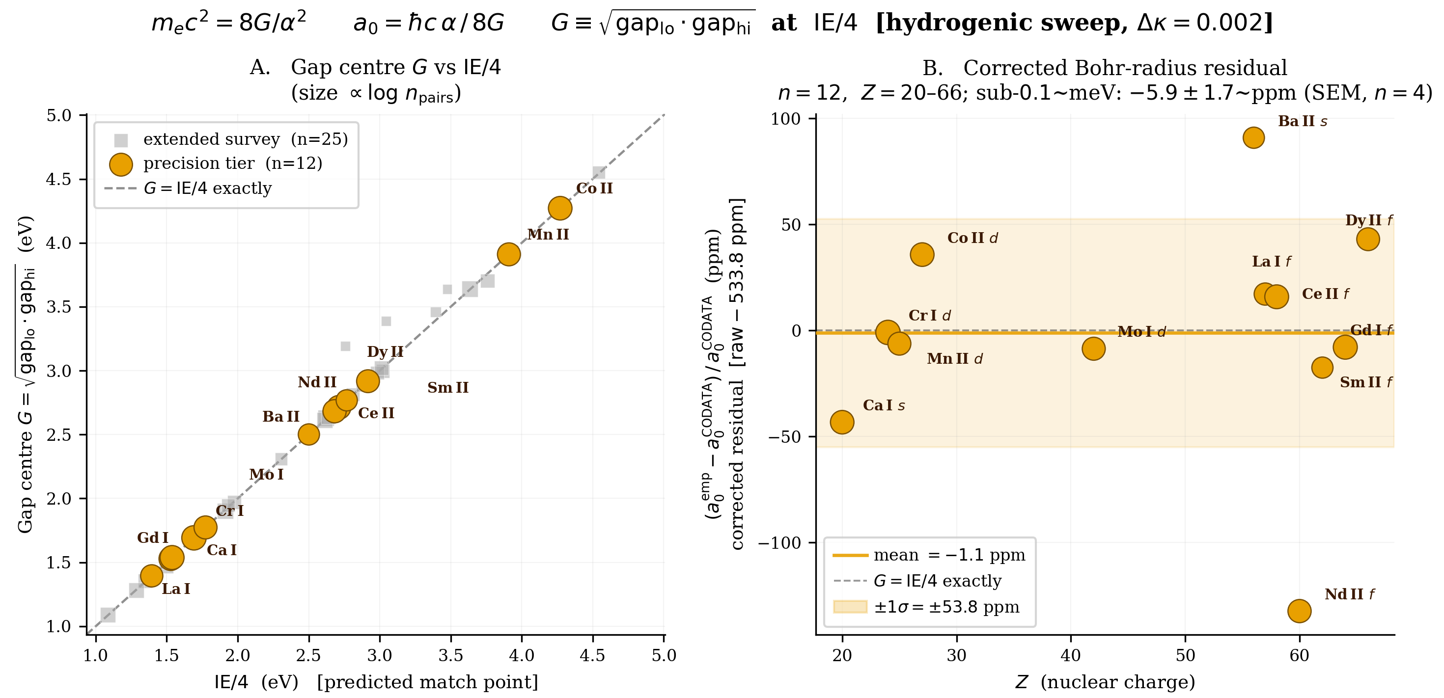
@ l r c c r r c r r @
Ion & \(Z\) & Fam. &
Gate\(^\dagger\) & Gap\(^\dagger\) & Rank\(^\dagger\) & Gate\(^\ddagger\) & Gap\(^\ddagger\) & Pairs\(^\ddagger\)
Ion & \(Z\) & Fam. &
Gate\(^\dagger\) & Gap\(^\dagger\) & Rank\(^\dagger\) & Gate\(^\ddagger\) & Gap\(^\ddagger\) & Pairs\(^\ddagger\)
H i & 1 & \(H\) & \(\star\) & & — & — & —
Li i & 3 & \(sp\) & \(\cdot\) & — & — & — & —
& —
N i & 7 & \(sp\) & \(\checkmark\)& \(30.3\) meV & \(0.0\)% & — & — & —
O i & 8 & \(sp\) & \(\cdot\) & — & — & — & —
& —
Na i & 11 & \(sp\) & \(\checkmark\)& \(8.6\) meV & \(0.5\)% & — & — & —
Mg i & 12 & \(sp\) & \(\checkmark\)& \(29.4\) meV & \(0.0\)% & — & — & —
Mg ii & 12 & \(sp\) & \(\checkmark\)& \(400.3\) meV & \(0.1\)% & — & — & —
Al i & 13 & \(sp\) & \(\checkmark\)& \(101.1\) meV & \(0.0\)% & — & — & —
P i & 15 & \(sp\) & \(\checkmark\)& \(19.2\) meV & \(0.1\)% & — & — & —
K i & 19 & \(sp\) & \(\checkmark\)& \(17.6\) meV & \(0.3\)% & \(\checkmark\)& \(13.9\) meV & 2,640
Ca i & 20 & \(sp\) & \(\checkmark\)& \(0.151\) meV & \(4.0\)% & — & — & —
Ca ii & 20 & \(sp\) & \(\cdot\) & — & — & — & —
& —
Sr ii & 38 & \(sp\) & \(\checkmark\)& \(1.4\) eV & \(1.7\)% & — & — & —
I i & 53 & \(sp\) & \(\checkmark\)& \(1.3\) meV & \(1.4\)% & — & — & —
Ba ii & 56 & \(sp\) & \(\checkmark\)& \(0.549\) meV & \(32.0\)% & \(\cdot\) & — &
3,476
Ti ii & 22 & \(d\) & \(\checkmark\)& \(306.1\) meV & \(9.2\)% & — & — & —
V ii & 23 & \(d\) & — & — & — & \(\checkmark\)& \(0.356\) meV & 31,000
Cr i & 24 & \(d\) & \(\checkmark\)& \(0.026\) meV & \(23.8\)% & \(\checkmark\)& \(0.345\) meV & 57,535
Cr ii & 24 & \(d\) & — & — & — & \(\checkmark\)& \(0.088\) meV &
160,145
Mn ii & 25 & \(d\) & \(\checkmark\)& \(0.052\) meV & \(41.3\)% & \(\checkmark\)& \(0.052\) meV & 63,134
Fe i & 26 & \(d\) & \(\checkmark\)& \(19.4\) meV & \(7.2\)% & \(\checkmark\)& \(0.088\) meV & 93,573
Fe ii & 26 & \(d\) & — & — & — & \(\checkmark\)& \(0.031\) meV &
198,667
Co ii & 27 & \(d\) & \(\checkmark\)& \(0.553\) meV & \(8.1\)% & \(\checkmark\)& \(0.553\) meV & 32,559
Ni ii & 28 & \(d\) & \(\checkmark\)& \(44.8\) meV & \(12.2\)% & — & — & —
Cu i & 29 & \(d\) & \(\checkmark\)& \(37.4\) meV & \(3.0\)% & — & — & —
Mo i & 42 & \(d\) & \(\checkmark\)& \(0.034\) meV & \(70.1\)% & \(\checkmark\)& \(0.034\) meV & 21,626
Au i & 79 & \(d\) & \(\checkmark\)& \(13.3\) meV & \(29.6\)% & — & — & —
La i & 57 & \(f\) & \(\checkmark\)& \(0.588\) meV & \(11.7\)% & \(\checkmark\)& \(0.588\) meV & 9,166
La ii & 57 & \(f\) & \(\checkmark\)& \(4.9\) meV & \(12.4\)% & — & — & —
Ce ii & 58 & \(f\) & \(\checkmark\)& \(0.110\) meV & \(18.3\)% & \(\checkmark\)& \(0.116\) meV & 46,678
Pr ii & 59 & \(f\) & \(\checkmark\)& \(1.8\) meV & \(13.3\)% & \(\checkmark\)& \(1.8\) meV & 2,198
Nd ii & 60 & \(f\) & \(\checkmark\)& \(0.735\) meV & \(1.6\)% & \(\checkmark\)& \(0.735\) meV & 25,373
Sm ii & 62 & \(f\) & \(\checkmark\)& \(0.327\) meV & \(42.4\)% & — & — & —
Eu ii & 63 & \(f\) & \(\checkmark\)& \(15.6\) meV & \(10.5\)% & \(\checkmark\)& \(15.6\) meV & 653
Gd i & 64 & \(f\) & \(\checkmark\)& \(0.091\) meV & \(11.0\)% & — & — & —
Gd ii & 64 & \(f\) & \(\checkmark\)& \(58.6\) meV & \(0.7\)% & \(\checkmark\)& \(0.262\) meV & 8,728
Tb ii & 65 & \(f\) & \(\checkmark\)& \(13.8\) meV & \(9.2\)% & \(\checkmark\)& \(13.8\) meV & 319
Dy ii & 66 & \(f\) & \(\checkmark\)& \(0.281\) meV & \(13.2\)% & \(\checkmark\)& \(0.281\) meV & 21,467
Ho i & 67 & \(f\) & \(\checkmark\)& \(2.5\) meV & \(6.5\)% & \(\checkmark\)& \(2.5\) meV & 1,725
Er ii & 68 & \(f\) & \(\checkmark\)& \(2.9\) meV & \(29.7\)% & \(\checkmark\)& \(2.9\) meV & 979
Tm ii & 69 & \(f\) & \(\checkmark\)& \(28.6\) meV & \(1.9\)% & — & — & —
Yb ii & 70 & \(f\) & \(\checkmark\)& \(1.1\) eV & \(11.4\)% & — & — & —
Lu ii & 71 & \(f\) & \(\checkmark\)& \(784.9\) meV & \(8.3\)% & — & — & —
| Ion | \(Z\) | Tier | Gap lo (meV) | Gap hi (meV) | Width (meV) | Pairs | Raw (ppm) | Corr. (ppm) |
|---|---|---|---|---|---|---|---|---|
| Fe ii | 26 | \(\star\) | 4046.920 | 4046.952 | 0.031 | 198,667 | \(+537.2\) | \(+3.4\) |
| Mo i | 42 | \(\star\) | 1773.098 | 1773.132 | 0.034 | 21,626 | \(+525.2\) | \(-8.6\) |
| Mn ii | 25 | \(\star\) | 3909.996 | 3910.052 | 0.056 | 63,134 | \(+527.6\) | \(-6.2\) |
| Fe i | 26 | \(\star\) | 1975.594 | 1975.682 | 0.088 | 93,573 | \(+527.2\) | \(-6.6\) |
| Cr ii | 24 | \(\star\) | 4121.373 | 4121.461 | 0.088 | 160,145 | \(+537.7\) | \(+3.9\) |
| Sub-\(0.1\) meV ensemble (\(n = 5\)) | \(531.0 \pm 6.0\) | \(-2.8 \pm 2.7\) | ||||||
| Ce ii | 58 | \(\bullet\) | 2712.477 | 2712.593 | 0.116 | 46,678 | \(+548.7\) | \(+14.9\) |
| Gd ii | 64 | \(\bullet\) | 3022.281 | 3022.543 | 0.262 | 8,728 | \(+562.9\) | \(+29.1\) |
| Dy ii | 66 | \(\bullet\) | 2917.234 | 2917.515 | 0.281 | 21,467 | \(+576.8\) | \(+43.0\) |
| Sub-\(0.3\) meV ensemble (\(n = 8\)) | \(543.0 \pm 18.7\) | \(+9.1 \pm 6.6\) | ||||||
| Cr i | 24 | \(\cdot\) | 1691.317 | 1691.662 | 0.345 | 57,535 | \(+614.2\) | \(+80.4\) |
| V ii | 23 | \(\cdot\) | 3658.333 | 3658.689 | 0.356 | 31,000 | \(+530.8\) | \(-3.0\) |
| Co ii | 27 | \(\cdot\) | 4270.671 | 4271.224 | 0.553 | 32,559 | \(+569.6\) | \(+35.8\) |
| La i | 57 | \(\cdot\) | 1393.907 | 1394.495 | 0.588 | 9,166 | \(+551.0\) | \(+17.2\) |
| Nd ii | 60 | \(\cdot\) | 2681.987 | 2682.722 | 0.735 | 25,373 | \(+401.5\) | \(-132.3\) |
| All precision (\(n = 13\)) | \(539.3 \pm 48.5\) | \(+5.5 \pm 13.5\) | ||||||
| Ion | \(Z\) | Width\(_\mathrm{0005}\) (meV) | Width\(_\mathrm{002}\) (meV) | Corr.\(_\mathrm{0005}\) (ppm) | Corr.\(_\mathrm{002}\) (ppm) |
|---|---|---|---|---|---|
| Fe ii | 26 | 0.031 | —\(^\dagger\) | \(+3.4\) | — |
| Mo i | 42 | 0.034 | 0.034 | \(-8.6\) | \(-8.6\) |
| Mn ii | 25 | 0.056 | 0.056 | \(-6.2\) | \(-6.2\) |
| Fe i | 26 | 0.088 | 19.4 | \(-6.6\) | —\(^\ddagger\) |
| Cr ii | 24 | 0.088 | —\(^\dagger\) | \(+3.9\) | — |
| Cr i | 24 | 0.345 | 0.026\(^\S\) | \(+80.4\) | \(-0.9\) |
@ l r c r r r c @
Ion & \(Z\) & Fam. & EH
& pos & Gap width & Flag
Ion & \(Z\) & Fam. & EH
& pos & Gap width & Flag
H i & 1 & \(H\) & \(0.001\) & \(0.001\) & \(6.8\) eV & \(\downarrow\)H
He i & 2 & \(H\) & \(0.098\) & \(0.089\) & \(15.0\) eV & —
He ii & 2 & \(H\) & \(0.056\) & \(0.053\) & \(28.7\) eV & —
Li i & 3 & \(sp\) & \(0.028\) & \(0.027\) & \(119.5\) meV & \(\downarrow\)H
C iv & 6 & \(sp\) & \(0.013\) & \(0.013\) & \(2.0\) eV & \(\downarrow\)H
N i & 7 & \(sp\) & \(0.016\) & \(0.016\) & \(3.5\) eV & \(\downarrow\)H
O i & 8 & \(sp\) & \(0.150\) & \(0.131\) & \(364.0\) meV & —
O iii & 8 & \(sp\) & \(48.96\) & \(0.980\) & \(385.7\) meV & \(\uparrow\)E
O vi & 8 & \(sp\) & \(14.07\) & \(0.934\) & \(7.3\) eV & —
Na i & 11 & \(sp\) & \(14.50\) & \(0.935\) & \(11.8\) meV & —
Mg i & 12 & \(sp\) & \(0.829\) & \(0.453\) & \(92.1\) meV & \(\leftrightarrow\)
Mg ii & 12 & \(sp\) & \(1.752\) & \(0.637\) & \(396.6\) meV & —
Al i & 13 & \(sp\) & \(2.183\) & \(0.686\) & \(121.9\) meV & —
P i & 15 & \(sp\) & \(0.066\) & \(0.062\) & \(2.1\) eV & \(\downarrow\)H
P v & 15 & \(sp\) & \(0.901\) & \(0.474\) & \(4.1\) eV & \(\leftrightarrow\)
K i & 19 & \(sp\) & \(2.019\) & \(0.669\) & \(37.2\) meV & —
Ca i & 20 & \(sp\) & \(0.166\) & \(0.142\) & \(190.7\) meV & —
Ca ii & 20 & \(sp\) & \(0.418\) & \(0.295\) & \(68.8\) meV & —
Sr ii & 38 & \(sp\) & \(0.393\) & \(0.282\) & \(67.3\) meV & —
I i & 53 & \(sp\) & \(0.408\) & \(0.290\) & \(34.2\) meV & —
Ba ii & 56 & \(sp\) & \(0.045\) & \(0.043\) & \(11.7\) meV & \(\downarrow\)H
Pb i & 82 & \(sp\) & \(0.411\) & \(0.292\) & \(189.5\) meV & —
Sc ii & 21 & \(d\) & \(1.035\) & \(0.509\) & \(6.0\) meV & \(\leftrightarrow\)
Ti ii & 22 & \(d\) & \(1.479\) & \(0.597\) & \(10.1\) meV & —
V ii & 23 & \(d\) & \(2.946\) & \(0.747\) & \(0.970\) meV & —
Cr i & 24 & \(d\) & \(0.548\) & \(0.354\) & \(2.2\) meV & —
Cr ii & 24 & \(d\) & \(26.51\) & \(0.964\) & \(3.3\) meV & \(\uparrow\)E
Mn i & 25 & \(d\) & \(1.711\) & \(0.631\) & \(115.9\) meV & —
Mn ii & 25 & \(d\) & \(7.908\) & \(0.888\) & \(1.6\) meV & —
Fe i & 26 & \(d\) & \(1.113\) & \(0.527\) & \(2.9\) meV & \(\leftrightarrow\)
Co ii & 27 & \(d\) & \(8.327\) & \(0.893\) & \(6.7\) meV & —
Ni i & 28 & \(d\) & \(880.5\) & \(0.999\) & \(12.7\) meV & \(\uparrow\)E
Ni ii & 28 & \(d\) & \(1.243\) & \(0.554\) & \(384.7\) meV & —
Cu i & 29 & \(d\) & \(6.053\) & \(0.858\) & \(3.7\) meV & —
Cu ii & 29 & \(d\) & \(6.771\) & \(0.871\) & \(10.1\) meV & —
Zn ii & 30 & \(d\) & \(0.020\) & \(0.019\) & \(337.1\) meV & \(\downarrow\)H
Nb i & 41 & \(d\) & \(2.438\) & \(0.709\) & \(5.7\) meV & —
Mo i & 42 & \(d\) & \(5.238\) & \(0.840\) & \(2.6\) meV & —
Ag i & 47 & \(d\) & \(0.257\) & \(0.204\) & \(105.4\) meV & —
Cd ii & 48 & \(d\) & \(12.56\) & \(0.926\) & \(74.7\) meV & —
Au i & 79 & \(d\) & \(2.291\) & \(0.696\) & \(164.1\) meV & —
Hg ii & 80 & \(d\) & \(0.572\) & \(0.364\) & \(45.4\) meV & —
La ii & 57 & \(f\) & \(1.433\) & \(0.589\) & \(40.9\) meV & —
Ce ii & 58 & \(f\) & \(0.788\) & \(0.441\) & \(3.8\) meV & \(\leftrightarrow\)
Ce iii & 58 & \(f\) & \(14.24\) & \(0.934\) & \(32.0\) meV & —
Pr ii & 59 & \(f\) & \(0.310\) & \(0.237\) & \(20.3\) meV & —
Nd ii & 60 & \(f\) & \(0.978\) & \(0.495\) & \(28.3\) meV & \(\leftrightarrow\)
Pm ii & 61 & \(f\) & \(0.830\) & \(0.454\) & \(21.4\) meV & \(\leftrightarrow\)
Sm ii & 62 & \(f\) & \(0.013\) & \(0.013\) & \(3.5\) meV & \(\downarrow\)H
Eu i & 63 & \(f\) & \(2.426\) & \(0.708\) & \(8.8\) meV & —
Eu ii & 63 & \(f\) & \(2.705\) & \(0.730\) & \(8.0\) meV & —
Gd i & 64 & \(f\) & \(0.080\) & \(0.074\) & \(40.5\) meV & \(\downarrow\)H
Gd ii & 64 & \(f\) & \(5.305\) & \(0.841\) & \(9.2\) meV & —
Tb i & 65 & \(f\) & \(0.235\) & \(0.190\) & \(43.0\) meV & —
Tb ii & 65 & \(f\) & \(1.169\) & \(0.539\) & \(27.2\) meV & —
Dy i & 66 & \(f\) & \(0.185\) & \(0.156\) & \(52.4\) meV & —
Dy ii & 66 & \(f\) & \(0.185\) & \(0.156\) & \(34.5\) meV & —
Ho i & 67 & \(f\) & \(0.635\) & \(0.388\) & \(105.7\) meV & —
Ho ii & 67 & \(f\) & \(0.207\) & \(0.171\) & \(41.6\) meV & —
Er i & 68 & \(f\) & \(0.772\) & \(0.436\) & \(27.5\) meV & \(\leftrightarrow\)
Er ii & 68 & \(f\) & \(2.598\) & \(0.722\) & \(33.6\) meV & —
Er iii & 68 & \(f\) & \(0.697\) & \(0.411\) & \(66.6\) meV & \(\leftrightarrow\)
Tm i & 69 & \(f\) & \(0.353\) & \(0.261\) & \(0.604\) meV & —
Tm ii & 69 & \(f\) & \(0.149\) & \(0.130\) & \(102.2\) meV & —
Yb ii & 70 & \(f\) & \(0.038\) & \(0.037\) & \(134.3\) meV & \(\downarrow\)H
Lu ii & 71 & \(f\) & \(4.503\) & \(0.818\) & \(66.9\) meV & —
| Family | \(n\) | Median EH | IQR | Median pos | MW \(p\) (vs \(sp\)) |
|---|---|---|---|---|---|
| Hydrogenic | 3 | \(0.056\) | \([0.028,\;0.077]\) | \(0.053\) | \(0.002^\dagger\) |
| \(s/p\)-block | 24 | \(0.385\) | \([0.055,\;1.114]\) | \(0.278\) | — (reference) |
| \(f\)-block | 20 | \(0.780\) | \([0.201,\;1.724]\) | \(0.438\) | \(0.88\) (n.s.) |
| \(d\)-block | 20 | \(2.365\) | \([1.093,\;7.055]\) | \(0.703\) | \(0.001\) |
| \(d > f\): \(p = 0.006\); H-like \(< d\): \(p = 0.002\). | |||||
| Test | \(r\) | \(p\) | \(n\) | Interpretation |
|---|---|---|---|---|
| Level-pair EH vs gap EH (primary) | \(-0.103\) | \(0.420\) | 63 | Not correlated |
| Level-pair EH vs line density EH | \(-0.058\) | \(0.668\) | 57 | Not correlated |
| Line density EH vs gap EH | \(-0.117\) | \(0.386\) | 57 | Not correlated |
@ l r r c r r r r @
Nuclide & \(Z\) & \(N\) & Gate & \(S_n/4\) (keV) & \(n_\downarrow\) & \(E_1\) (keV) & \(\kappa_\mathrm{nuc}\)
Nuclide & \(Z\) & \(N\) & Gate & \(S_n/4\) (keV) & \(n_\downarrow\) & \(E_1\) (keV) & \(\kappa_\mathrm{nuc}\)
\(^{16}\)O & 8 & 8 & \(\checkmark\checkmark\) & 3916 & 0
& 6049 & \(0.1934\)
\(^{48}\)Ca & 20 & 28 &
\(\checkmark\checkmark\) & 2488
& 0 & 3832 & \(0.1940\)
\(^{132}\)Sn & 50 & 82 &
\(\checkmark\checkmark\) & 1838
& 0 & 4041 & \(0.1217\)
\(^{208}\)Pb & 82 &126 &
\(\checkmark\checkmark\) & 1842
& 0 & 2615 & \(0.2106\)
\(^{12}\)C & 6 & 6 & \(\checkmark\) & 4680 & 1 & 7654
& \(0.1818\)
\(^{209}\)Pb & 82 &127 &
\(\checkmark\) & 984 & 1 &
1423 & \(0.2069\)
\(^{40}\)K & 19 & 21 &
\(\checkmark\) & 1950 & 4 &
1959 & \(0.2808\)
\(^{56}\)Ni & 28 & 28 &
\(\checkmark\) & 4161 & 3 &
4932 & \(0.2472\)
\(^{60}\)Co & 27 & 33 &
\(\checkmark\) & 1873 & 36
& 1877 & \(0.2813\)
\(^{98}\)Mo & 42 & 56 &
\(\checkmark\) & 2161 & 11
& 2207 & \(0.2775\)
\(^{139}\)La & 57 & 82 &
\(\checkmark\) & 2194 & 40
& 2232 & \(0.2783\)
\(^{238}\)U & 92 &146 &
\(\checkmark\) & 1539 & 54
& 1546 & \(0.2808\)
\(^{22}\)Na & 11 & 11 &
\(\star\) & 2767 & 9 & 2969
& \(0.2675\)
\(^{56}\)Fe & 26 & 30 &
\(\star\) & 2799 & 3 & 2942
& \(0.2717\)
\(^{56}\)Co & 27 & 29 &
\(\star\) & 2520 & 19 &
2610 & \(0.2747\)
\(^{57}\)Co & 27 & 30 &
\(\star\) & 2844 & 21 &
2879 & \(0.2793\)
\(^{58}\)Ni & 28 & 30 &
\(\star\) & 3054 & 6 & 3264
& \(0.2683\)
\(^{90}\)Zr & 40 & 50 &
\(\star\) & 2992 & 5 & 3077
& \(0.2761\)
\(^{140}\)Ce & 58 & 82 &
\(\star\) & 2300 & 4 & 2348
& \(0.2776\)
\(^{133}\)Ba & 56 & 77 &
\(\times\) & 1797 & 42 &
1830 & \(0.2781\)
\(^{137}\)Cs & 55 & 82 &
\(\times\) & 2070 & 15 &
2099 & \(0.2788\)
\(^{141}\)Pr & 59 & 82 &
\(\times\) & 2350 & 70 &
2354 & \(0.2814\)
\(^{151}\)Sm & 62 & 89 &
\(\times\) & 1399 &130 &
1409 & \(0.2803\)
\(^{153}\)Eu & 63 & 90 &
\(\times\) & 2138 &122 &
2182 & \(0.2775\)
\(^{155}\)Gd & 64 & 91 &
\(\times\) & 1609 &146 &
1615 & \(0.2809\)
\(^{156}\)Gd & 64 & 92 &
\(\times\) & 2134 & 84 &
2134 & \(0.2817\)
\(^{157}\)Gd & 64 & 93 &
\(\times\) & 1590 &124 &
1607 & \(0.2796\)
\(^{158}\)Gd & 64 & 94 &
\(\times\) & 1984 & 61 &
1997 & \(0.2805\)
\(^{162}\)Dy & 66 & 96 &
\(\times\) & 2049 & 71 &
2054 & \(0.2813\)
\(^{163}\)Dy & 66 & 97 &
\(\times\) & 1568 &107 &
1572 & \(0.2812\)
\(^{165}\)Dy & 66 & 99 &
\(\times\) & 1429 & 70 &
1441 & \(0.2801\)
\(^{165}\)Ho & 67 & 98 &
\(\times\) & 1997 &118 &
2012 & \(0.2803\)
\(^{167}\)Er & 68 & 99 &
\(\times\) & 1609 &105 &
1625 & \(0.2798\)
\(^{169}\)Tm & 69 &100 &
\(\times\) & 2008 & 69 &
2076 & \(0.2751\)
\(^{170}\)Tm & 69 &101 &
\(\times\) & 1648 &165 &
1659 & \(0.2804\)
\(^{171}\)Yb & 70 &101 &
\(\times\) & 1654 & 91 &
1656 & \(0.2814\)
\(^{182}\)Ta & 73 &109 &
\(\times\) & 1516 &118 &
1527 & \(0.2802\)
\(^{192}\)Ir & 77 &115 &
\(\times\) & 1550 &174 &
1552 & \(0.2815\)
\(^{232}\)Th & 90 &142 &
\(\times\) & 1610 & 62 &
1618 & \(0.2807\)
\(^{17}\)O & 8 & 9 & \(\cdot\) & 1036 & 1 & — &
—
\(^{152}\)Eu & 63 & 89 &
\(\cdot\) & 1577 &189 & —
& —
\(^{154}\)Eu & 63 & 91 &
\(\cdot\) & 1611 &156 & —
& —
\(^{155}\)Eu & 63 & 92 &
\(\cdot\) & 2038 & 80 & —
& —
\(^{160}\)Tb & 65 & 95 &
\(\cdot\) & 1594 &119 & —
& —
\(^{166}\)Ho & 67 & 99 &
\(\cdot\) & 1561 &226 & —
& —
\(^{188}\)Re & 75 &113 &
\(\cdot\) & 1468 &171 & —
& —
\(^{197}\)Au & 79 &118 &
\(\cdot\) & 2018 & 32 & —
& —
\(^{226}\)Ra & 88 &138 &
\(\cdot\) & 1599 & 32 & —
& —
@ p0.29 p0.30 p0.37 @
Claim & Evidence & Falsification condition
Claim & Evidence & Falsification condition
Universal gap at \(\mathit{IE}/4\):
no observed photon transition carries the energy \(\mathit{IE}/4\) for any ion with sufficient
catalog coverage (§8) & 71/80 NIST ions confirmed; 0
falsified; gap rank at 92.5th percentile median across confirmed ions
& Any ion with \(\geq 200\)
observed lines spanning \(\mathit{IE}/4\) from both sides where a
line falls within \(1~\mathrm{meV}\) of
\(\mathit{IE}/4\)
\(\mathit{IE}/4\) is the unique
impedance-match fraction: the gap centre encodes \(m_e c^2\) only at \(\mathit{IE}/4\), not at other fractions
(§8.2) & \(\mathit{IE}/3\) returns \(-250{,}133 \pm 1.1~\mathrm{ppm}\) (SEM);
\(\mathit{IE}/5\) returns \(+250{,}129 \pm 4.6~\mathrm{ppm}\); \(\mathit{IE}/4\) returns \(-2.8 \pm 2.7~\mathrm{ppm}\) & Any wrong
fraction (\(\mathit{IE}/3\), \(\mathit{IE}/5\), etc.) returning a
corrected residual within \(\pm
50~\mathrm{ppm}\) under identical methodology with \(n \geq 4\) precision-tier ions
Gap centre at \(\mathit{IE}/4\):
\(G =
\sqrt{\mathrm{gap\_lo}\cdot\mathrm{gap\_hi}}
= \mathit{IE}/4\) to \(\pm\,2.7~\mathrm{ppm}\) (SEM) for
electromagnetically symmetric ions (§9) &
\(\delta_G^\mathrm{corr} = -2.8 \pm
2.7~\mathrm{ppm}\), \(n = 5\)
sub-\(0.1~\mathrm{meV}\) ions; \(+5.5 \pm 13.5~\mathrm{ppm}\), \(n = 13\) all precision & Mean \(|\delta_G^\mathrm{corr}| >
100~\mathrm{ppm}\) across \(\geq
10\) precision-tier ions all satisfying \(\mathrm{gap\_width} < 0.5~\mathrm{meV}\)
and \(\sigma_\mathrm{exp}/\Delta
E_\mathrm{step} < 1.0\)
Shell ordering of gap width: \(d\)-block gaps narrower than \(s/p\)-block; \(f\)-block intermediate (§8.4) & \(d\): median \(8.4~\mathrm{meV}\); \(f\): \(32.8~\mathrm{meV}\); \(sp\): \(189.5~\mathrm{meV}\); Mann-Whitney \(d < sp\), \(p
= 1.1\times10^{-4}\) & Mann-Whitney \(d < sp\) returning \(p > 0.05\) with \(n_d \geq 15\) and \(n_{sp} \geq 15\) confirmed ions, or \(d\)-block median exceeding \(f\)-block median
E/H partition stratifies by shell family: \(d\)-block EH ratio \(>\) \(f\)-block \(>\) \(s/p\)-block (§8.8) &
\(d\): median EH ratio \(= 2.365\); \(f\): \(0.780\); \(sp\): \(0.385\); Mann-Whitney \(f < d\), \(p =
0.006\) & Mann-Whitney \(f <
d\) on EH ratio returning \(p >
0.05\) with \(n_d \geq 15\) and
\(n_f \geq 15\) confirmed ions
EH ratio is not predicted by level-pair energy asymmetry: the
partition encodes transition geometry, not level density (§11.7) & \(r(\log\,\mathrm{EH_{levels}},\,\log\,\mathrm{EH_{lines}})
= -0.103\), \(p = 0.42\), \(n = 63\) & Spearman \(|r| > 0.4\) with \(p < 0.01\) in a survey of \(n \geq 50\) ions using the same
levels-vs-lines independence test
Orbital impedance formula \(Z_{\!\mathrm{orb}}(n) = Z_0\,n/\alpha\)
from Coulomb and Biot–Savart (§5) &
Mathematical derivation; \(Z_{\!\mathrm{orb}}(1) = 51{,}626~\Omega\)
verified numerically & An identified error in the derivation steps
\(Z_{\!\mathrm{orb}}=
|\mathcal{E}|/|\mathcal{H}|
= 1/\varepsilon_0 v_n = Z_0\,n/\alpha\)
Nuclear analogue at \(S_n/4\): all
four doubly magic nuclei show complete depletion; no non-doubly-magic
nuclide shows a gap (§11.8)
& \(n_\downarrow = 0\) for \(^{16}\)O, \(^{48}\)Ca, \(^{132}\)Sn, \(^{208}\)Pb; \(n_\downarrow \gg 0\) for all 20
non-doubly-magic nuclides & Any doubly magic nucleus with ENSDF
coverage \(> 200\%\) showing \(n_\downarrow \geq 3\) levels below \(S_n/4\), or any mid-shell nucleus showing
\(n_\downarrow = 0\) with coverage
\(> 100\%\)
An independent researcher can verify the central claims of this paper from raw NIST data using only the five-step procedure below. No pipeline code, no sweep configuration files, and no prior knowledge of \(m_e\) or \(a_0\) are required for steps 1–3. Steps 4 and 5 extend the verification to the precision measurement.
Step 1: The 30-second gap test (any ion).
Choose any ion with a published ionization energy and a NIST spectroscopic line catalog.
Download the NIST ASD line list for the ion (https://physics.nist.gov/asd, Lines form).
Compute \(\mathit{IE}/4\) in meV from the NIST sequential ionization energy.
Sort the catalog by photon energy in meV.
Find the two consecutive entries \(h\nu_j\) and \(h\nu_{j+1}\) that bracket \(\mathit{IE}/4\): confirm that \(h\nu_j < \mathit{IE}/4 < h\nu_{j+1}\).
This test requires no model, no \(\alpha\), and no coordinate system. If the gap does not exist for a well-covered ion, the primary claim is falsified.
Step 2: The uniqueness test (three fractions).
Download NIST energy levels for Fe ii (\(Z = 26\), \(\mathit{IE}= 16.1878~\mathrm{eV}\)). Form all pairwise level-energy differences \(\Delta E = E_k - E_i\) (\(E_k > E_i\)) and sort the resulting array. For each fraction \(f \in \{3, 4, 5\}\):
Compute the target \(\mathit{IE}/f\) in meV.
Locate \(\mathrm{gap\_lo} = \max\{\Delta E_j < \mathit{IE}/f\}\) and \(\mathrm{gap\_hi} = \min\{\Delta E_j > \mathit{IE}/f\}\).
Compute \(G = \sqrt{\mathrm{gap\_lo}\cdot\mathrm{gap\_hi}}\) and the raw fractional offset \(\delta = (G - \mathit{IE}/f)/(\mathit{IE}/f) \times 10^6\) ppm.
Subtract the reduced-mass baseline \(+533.8~\mathrm{ppm}\) to obtain the corrected residual.
Expected results (corrected):
| Fraction | Algebraic prediction | Expected result |
|---|---|---|
| \(\mathit{IE}/3\) | \(+250{,}000\) ppm | \(\approx +250{,}000\) ppm |
| \(\mathit{IE}/4\) | \(0\) ppm | \(\approx 0\) ppm (signal) |
| \(\mathit{IE}/5\) | \(-250{,}000\) ppm | \(\approx -250{,}000\) ppm |
If \(\mathit{IE}/4\) does not return near-zero while \(\mathit{IE}/3\) and \(\mathit{IE}/5\) return the expected \(\pm 250{,}000\) ppm, the uniqueness claim is falsified.
Step 3: The five headline ions.
Repeat Step 2 at \(\mathit{IE}/4\) only for the five sub-\(0.1~\mathrm{meV}\) headline ions. Required NIST ionization energies:
| Ion | Symbol | \(\mathit{IE}\) (eV) |
|---|---|---|
| Fe ii | Iron II | 16.1878 |
| Mo i | Molybdenum | 7.0924 |
| Mn ii | Manganese II | 15.6400 |
| Fe i | Iron I | 7.9025 |
| Cr ii | Chromium II | 16.4857 |
Individual corrected residuals should be within \(\pm 15~\mathrm{ppm}\) of the values in Table 1 if the ionization energies match those above. The mean across the five ions should be within \(\pm 15~\mathrm{ppm}\) of \(-2.8~\mathrm{ppm}\).
Step 4: Hydrogen by arithmetic alone.
No NIST data, no pipeline, no constants beyond \(E_0 = 13.6057~\mathrm{eV}\).
Compute all transition energies \(\Delta E(n_f, n_i) = E_0(1/n_f^2 - 1/n_i^2)\) for \(1 \leq n_f < n_i \leq 40\).
Confirm that none satisfies \(\Delta E = E_0/4 = \mathit{IE}/4\); i.e., that \(1/n_f^2 - 1/n_i^2 = 1/4\) has no solution in positive integers with \(n_f < n_i \leq 40\).
Confirm that the 518 NIST H i lines distribute as: 440 lines in \([0,\,\mathit{IE}/4)\); 0 lines in \([\mathit{IE}/4,\,3\mathit{IE}/4)\); 76 lines in \([3\mathit{IE}/4,\,\mathit{IE})\). (The two Lyman-\(\alpha\) fine-structure components at \(10{,}198.806\) and \(10{,}198.811~\mathrm{meV}\) straddle \(3\mathit{IE}/4 = 10{,}198.826~\mathrm{meV}\) by \(< 0.02~\mathrm{meV}\) and are not exceptions to the partition.)
Step 5: The hydrogenic ruler and self-consistency.
Using the coordinate \(\kappa(\Delta E;\,Z) = \log_{10}(\Delta E/E_0 Z^2)\,/\,\log_{10}\alpha\) (equation [eq:kappa]), confirm the following for the analytic hydrogen template (\(E_n = E_0/n^2\), \(1 \leq n_f < n_i \leq 60\)):
Assign each of the \(\binom{60}{2} = 1{,}770\) pairs to the nearest \(\kappa\) bin at step \(\Delta\kappa = 0.002\).
The bin at \(\kappa = 0.2820\) (nearest to \(\kappa_{\mathrm{q}}= 0.2818\)) should contain 35 coincidences, all of the form \((n_f = 2,\, n_i \geq 26)\), with mean \(\Delta E \approx 3{,}393~\mathrm{meV}\) converging toward \(\mathit{IE}/4 = 3{,}401~\mathrm{meV}\).
The bin at \(\kappa = 0.0000\) should contain 46 coincidences of the form \((n_f = 1,\, n_i \geq 15)\), confirming that the two dominant accumulation points of the hydrogen spectrum — Lyman and Balmer series limits — fall at \(\kappa = 0\) and \(\kappa = \kappa_{\mathrm{q}}\) respectively.
These results confirm that the hydrogenic ruler locates the impedance boundary at the correct coordinate without any free parameter.
Data and code availability.
NIST spectroscopic data: https://physics.nist.gov/asd.
ENSDF nuclear data: https://www.nndc.bnl.gov/ensdf/.
The complete ion manifest, YAML sweep configuration files, pipeline
scripts, and all intermediate analysis files are available from the
corresponding author on request. All numerical results in this paper are
derived solely from these publicly available data sources and CODATA
2018 physical constants; no proprietary data or model outputs are
involved.
The research that gave rise to this paper was conducted by Kelly
B. Heaton through an interactive collaboration with Claude (Sonnet 4.6,
a large language model developed by Anthropic), and ChatGPT (large
language models developed by OpenAI), collectively referred to as the
Coherence Research Collaboration. All research design, direction,
interpretation, and conclusions were determined by the human author who
is the sole owner of the intellectual property. DOI:
10.5281/zenodo.19164224
v1.0: March 2026. Initial publication.
v1.1: March 2026. Corrected citation metadata for Heaton (2026c):
updated title to The Encounter of Two Primitives and One Flaw: Geometric
Unification at the Electromagnetic Scale, updated status from
forthcoming to published, and corrected DOI URL. No changes to
scientific content.
Follow the light of the lantern.